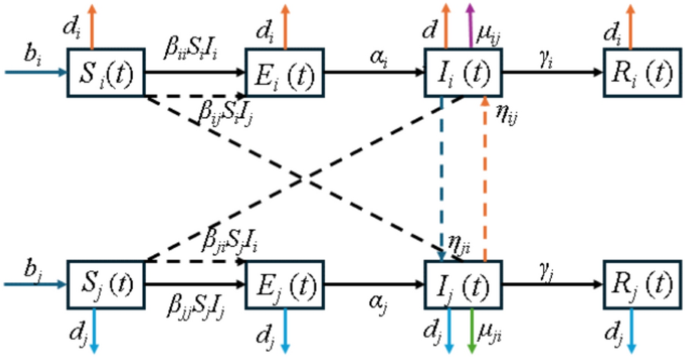
Properties of solutions
Lemma 1
The positive invariant set of the system (4) with positive invariant set is as follows.
$$\begin{gathered} \Omega = \left\{ {\left( {S_{1} \left( t \right),E_{1} \left( t \right),I_{1} \left( t \right),R_{1} \left( t \right),S_{2} \left( t \right),E_{2} \left( t \right),I_{2} \left( t \right),R_{2} \left( t \right)} \right) \in {\mathbf{R}}_{ + }^{8} \left| {S_{i} \left( t \right)} \right.} \right. \hfill \\ \left. { + E_{i} \left( t \right) + I_{i} \left( t \right) + R_{i} \left( t \right) < \frac{{b_{i} }}{{\delta_{i} }},i = 1,2} \right\} \hfill \\ \end{gathered}$$
Proof Based on the four equations of the system (4) and let \(\varepsilon_{i} = \min \left[ {d_{1} ,\left( {\mu_{12} + d_{1} + \eta_{21} } \right)} \right]\), so we have that
$$\begin{gathered} \frac{{{\text{d}}S_{i} \left( t \right)}}{{{\text{d}}t}} + \frac{{{\text{d}}E_{i} \left( t \right)}}{{{\text{d}}t}} + \frac{{{\text{d}}I_{i} \left( t \right)}}{{{\text{d}}t}} + \frac{{{\text{d}}R_{i} \left( t \right)}}{{{\text{d}}t}} \hfill \\ = b_{i} + \eta_{ij} I_{i} \left( t \right) – d_{i} \left( {S_{i} \left( t \right) + E_{i} \left( t \right) + R_{i} \left( t \right)} \right) – \left( {\mu_{ij} + d_{i} + \eta_{ji} } \right)I_{i} \left( t \right) \hfill \\ \le b_{i} – d_{i} \left( {S_{i} \left( t \right) + E_{i} \left( t \right) + R_{i} \left( t \right)} \right) – \left( {\mu_{ij} + d_{i} + \eta_{ji} } \right)I_{i} \left( t \right) \hfill \\ \le b_{i} – \varepsilon_{i} \left( {S_{i} \left( t \right) + E_{i} \left( t \right) + I_{i} \left( t \right) + R_{i} \left( t \right)} \right),i = 1,2. \hfill \\ \end{gathered}$$
(5)
There by obtaining
$$\mathop {\lim }\limits_{t \to + \infty } \sup S_{i} \left( t \right) + E_{i} \left( t \right) + I_{i} \left( t \right) + R_{i} \left( t \right) \le \frac{{b_{i} }}{{\varepsilon_{i} }},i = 1,2.$$
This implies that the feasible region \(\Omega\) is orthogonally invariant for system (4).
Lemma 2
For all \(t > 0\) and \(i = 1,2\) , the solutions \(S_{i} \left( t \right)\), \(E_{i} \left( t \right)\), \(I_{i} \left( t \right)\), \(R_{i} \left( t \right)\) of system (4) with initial conditions \(S_{i} \left( 0 \right) > 0\), \(E_{i} \left( 0 \right) > 0\), \(I_{i} \left( 0 \right) > 0\), \(R_{i} \left( 0 \right) > 0\) are positive.
Proof
From the initial conditions of system (1), we know that \(S_{i} \left( 0 \right) > 0\), \(E_{i} \left( 0 \right) > 0\), \(I_{i} \left( 0 \right) > 0\), \(R_{i} \left( 0 \right) > 0\), \(i = 1,2\).
indicate
$$h\left( t \right) = \mathop {\min }\limits_{t} \left\{ {S_{i} \left( 0 \right),E_{i} \left( 0 \right), I_{i} \left( 0 \right),R_{i} \left( 0 \right),i = 1,2} \right\}.$$
All we need to do to prove that \(S_{i} \left( t \right)\), \(E_{i} \left( t \right)\), \(I_{i} \left( t \right)\), and \(R_{i} \left( t \right)\) are positive at any \(t > 0\) moment is to prove that \(h\left( t \right) > 0\) is positive at any \(t > 0\) moment. Based on reductio ad absurdum, assume that there exists a positive number \(t_{1}\) such that.
\(h\left( {t_{1} } \right) = 0\), and when \(t \in \left( {0,t_{1} } \right)\),\(h\left( t \right) > 0\).
Below we discuss the function \(h\left( t \right)\) in four cases.
Suppose there exists a positive integer \(i_{1} \in \left\{ {1,2} \right\}\) such that \(h\left( {t_{1} } \right) = S_{{i_{1} }} \left( {t_{1} } \right) = 0\). From system (4) we know that:
$$\frac{{{\text{d}}S_{i1} \left( t \right)}}{{{\text{d}}t}} = b_{i1} – \beta_{i1} S_{i1} \left( t \right)I_{i1} \left( t \right) – \beta_{i1}^{\prime } S_{i1} \left( t \right)I_{i1}^{\prime } \left( t \right) – d_{i1} S_{i1} \left( t \right),$$
when \(t = t_{1}\), and by substituting the assumption \(S_{{i_{1} }} \left( {t_{1} } \right) = 0\) into the above formula, we obtain the following:
$$\frac{{{\text{d}}S_{{i_{1} }} \left( t \right)}}{{{\text{d}}t}}\left| {_{{t = t_{1} }} } \right. = b_{{_{{i_{1} }} }} > 0$$
This is consistent with the assumption \(S_{{i_{1} }} \left( {t_{1} } \right) = 0\) and the premise that \(S_{{i_{1} }} \left( t \right)\) begins to decrease at \(t = t_{1}\). Therefore,\(S_{{i_{1} }} \left( t \right)\) is always positive when \(t > 0\).
Suppose there exists a positive integer \(i_{1} \in \left\{ {1,2} \right\}\) such that \(h\left( {t_{1} } \right) = E_{{i_{1} }} \left( {t_{1} } \right)\). From system (4) we know that:
$$\frac{{{\text{d}}E_{i1} \left( t \right)}}{{{\text{d}}t}} = \beta_{i1} S_{i1} \left( t \right)I_{i1} \left( t \right) + \beta_{i1}^{\prime } S_{i1} \left( t \right)I_{i1}^{\prime } \left( t \right) – \alpha_{1} E_{i1} \left( t \right) – d_{1} E_{i1} \left( t \right),$$
when \(t = t_{1}\), and by substituting the assumption \(E_{{i_{1} }} \left( {t_{1} } \right) = 0\) into the above formula, we obtain the following:
$$\frac{{{\text{d}}E_{i1} \left( t \right)}}{{{\text{d}}t}}\left| {t = t_{1} } \right. = \beta_{i1} S_{i1} \left( t \right)I_{i1} \left( t \right) + \beta_{i1}^{\prime } S_{i1} \left( t \right)I_{i1}^{\prime } \left( t \right),$$
therefore \(S_{{i_{1} }} \left( t \right) \ge 0\), \(I_{{i_{1} }} \left( t \right) \ge 0\) and \(I_{{i_{1}^{\prime } }} \left( t \right) \ge 0\), \(\beta_{{i_{1} }} > 0\), \(\beta^{\prime}_{{i_{1} }} > 0\),so.
\(\frac{{{\text{d}}E_{{i_{1} }} \left( t \right)}}{{{\text{d}}t}}\left| {_{{t = t_{1} }} } \right. > 0\).
This is consistent with the assumption \(E_{{i_{1} }} \left( {t_{1} } \right) = 0\) and the premise that \(E_{{i_{1} }} \left( t \right)\) begins to decrease at \(t = t_{1}\). Therefore,\(E_{{i_{1} }} \left( t \right)\) is always positive when \(t > 0\).
Suppose there exists a positive integer \(i_{1} \in \left\{ {1,2} \right\}\) such that \(h\left( {t_{1} } \right) = I_{{i_{1} }} \left( {t_{1} } \right)\). From system (4) we know that:
$$\frac{{{\text{d}}I_{i} \left( t \right)}}{{{\text{d}}t}} = \alpha_{i1} E_{i1} \left( t \right) – \left( {\gamma_{i1} + \mu_{{i1i^{\prime}_{1} }} + \eta_{{i^{\prime}_{1} i1}} + d_{i1} } \right)I_{i1} \left( t \right) + \eta_{{i^{\prime}_{1} i1}} I_{i1}^{\prime } \left( t \right),$$
when \(t = t_{1}\), and by substituting the assumption \(I_{{i_{1} }} \left( {t_{1} } \right) = 0\) into the above formula, we obtain the following:
$$\frac{{{\text{d}}I_{{i_{1} }} \left( t \right)}}{{{\text{d}}t}}\left| {_{{t = t_{1} }} } \right. = \alpha_{{i_{1} }} E_{{i_{1} }} \left( t \right),$$
therefore \(E_{{i_{1} }} \left( t \right) \ge 0\) and \(\alpha_{{i_{1} }} > 0\),so.
\(\frac{{{\text{d}}I_{{i_{1} }} \left( t \right)}}{{{\text{d}}t}}\left| {t = t_{1} } \right. > 0\).
This is consistent with the assumption \(I_{{i_{1} }} \left( {t_{1} } \right) = 0\) and the premise that \(I_{{i_{1} }} \left( t \right)\) begins to decrease at \(t = t_{1}\). Therefore,\(I_{{i_{1} }} \left( t \right)\) is always positive when \(t > 0\).
Suppose there exists a positive integer \(i_{1} \in \left\{ {1,2} \right\}\) such that \(h\left( {t_{1} } \right) = R_{i1} \left( {t_{1} } \right)\). From system (4) we know that:
$$\frac{{{\text{d}}R_{i1} \left( t \right)}}{{{\text{d}}t}} = \gamma_{i1} I_{i1} \left( t \right) – d_{i1} R_{i1} \left( t \right),$$
when \(t = t_{1}\), and by substituting the assumption \(R_{{i_{1} }} \left( {t_{1} } \right) = 0\) into the above formula, we obtain the following:
$$\frac{{{\text{d}}R_{i1} \left( t \right)}}{{{\text{d}}t}} = \gamma_{i1} I_{i1} \left( t \right),$$
therefore, \(I_{i1} \left( t \right) \ge 0\) and,\(\gamma_{i1} > 0\), so.
\(\frac{{{\text{d}}R_{i1} \left( t \right)}}{{{\text{d}}t}}\left| {t = t_{1} } \right. > 0\).
This is consistent with the assumption \(R_{{i_{1} }} \left( {t_{1} } \right) = 0\) and the premise that \(R_{{i_{1} }} \left( t \right)\) begins to decrease at \(t = t_{1}\). Therefore,\(R_{{i_{1} }} \left( t \right)\) is always positive when \(t > 0\).
Thus we have that the solution \(S_{i} \left( t \right)\), \(E_{i} \left( t \right)\), \(I_{i} \left( t \right)\), \(R_{i} \left( t \right)\) of system (4) with initial conditions \(S_{i} \left( 0 \right) > 0\), \(E_{i} \left( 0 \right) > 0\), \(I_{i} \left( 0 \right) > 0\), \(R_{i} \left( 0 \right) > 0\) is positive for all \(t > 0\) and \(i = 1,2\).
Basic regeneration number
It is easy to see that model (4) has a disease-free equilibrium point as shown below:
$$E^{0} = \left( {S_{1}^{0} ,0,0,0,S_{2}^{0} ,0,0,0} \right),S_{i}^{0} = \frac{{b_{i} }}{{d_{i} }},i = 1,2$$
Define the endemic disease equilibrium points within \(\Omega\) as \(E^{*} = \left( {S_{1}^{*} ,E_{1}^{*} ,I_{1}^{*} ,R_{1}^{*} ,S_{2}^{*} ,E_{2}^{*} ,I_{2}^{*} ,R_{2}^{*} } \right)\).
Next, the familiar next-generation matrix method is utilized to find the fundamental regeneration number of system (4). We define the vector \(\chi = \left( {S_{1} ,S_{2} ,E_{1} ,E_{2} ,I_{1} ,I_{2} ,R_{1} ,R_{2} } \right)^{T}\). From this we obtain the \(8 \times 8\) matrices \(F\), \(V\), \(V^{ – 1}\) of:
$$F = \left( {\begin{array}{*{20}c} 0 & 0 & {F_{1} } & 0 \\ 0 & 0 & 0 & 0 \\ 0 & 0 & 0 & 0 \\ 0 & 0 & 0 & 0 \\ \end{array} } \right),\;V = \left( {\begin{array}{*{20}c} {V_{1} } & 0 & 0 & 0 \\ 0 & {V_{2} } & {V_{3} } & 0 \\ 0 & 0 & {V_{4} } & 0 \\ 0 & 0 & {V_{5} } & {V_{6} } \\ \end{array} } \right),\;V^{ – 1} = \left( {\begin{array}{*{20}c} {M_{1} } & 0 & 0 & 0 \\ 0 & {M_{2} } & {M_{3} } & 0 \\ 0 & 0 & {M_{4} } & 0 \\ 0 & 0 & {M_{5} } & {M_{6} } \\ \end{array} } \right)$$
Among them \(F_{1} = \left( {\begin{array}{*{20}c} {\beta_{11} S_{1} } & {\beta_{12} S_{1} } \\ {\beta_{21} S_{2} } & {\beta_{22} S_{2} } \\ \end{array} } \right)\), \(V_{1} = diag\left\{ { – d_{1} , – d_{2} } \right\}\), \(V_{2} = diag\left\{ {\alpha_{1} + d_{1} ,\alpha_{2} + d_{2} } \right\}\), \(V_{3} = diag\left\{ { – \left( {\gamma_{1} + \mu_{12} + \eta_{21} } \right), – \left( {\gamma_{2} + \mu_{21} + \eta_{12} } \right)} \right\}\),\(V_{4} = diag\left\{ {\gamma_{1} + \mu_{12} + d_{1} ,\gamma_{2} + \mu_{21} + d_{2} } \right\}\), \(V_{5} = diag\left\{ {\eta_{21} ,\eta_{12} } \right\}\), \(V_{6} = diag\left\{ { – d_{1} , – d_{2} } \right\}\), \(M_{1} = diag\left\{ { – \frac{1}{{d_{1} }}, – \frac{1}{{d_{2} }}} \right\}\) ,\(M_{2} = diag\left\{ { – \frac{1}{{d_{1} + \alpha_{1} }}, – \frac{1}{{d_{2} + \alpha_{2} }}} \right\}\),\(M_{3} = diag\left\{ {\frac{{\mu_{12} + \gamma_{1} + \eta_{21} }}{{\left( {d_{1} + \alpha_{1} } \right)\left( {d_{1} + \mu_{12} + \gamma_{1} } \right)}},\frac{{\mu_{21} + \gamma_{2} + \eta_{12} }}{{\left( {d_{2} + \alpha_{2} } \right)\left( {d_{2} + \mu_{21} + \gamma_{2} } \right)}}} \right\}\),\(M_{4} = diag\left\{ {\frac{1}{{d_{1} + \mu_{12} + \gamma_{1} }},\frac{1}{{d_{2} + \mu_{21} + \gamma_{2} }}} \right\}\), \(M_{5} = diag\left\{ {\frac{{\eta_{21} }}{{d_{1} \left( {d_{1} + \mu_{12} + \gamma_{1} } \right)}},\frac{{\eta_{12} }}{{d_{2} \left( {d_{2} + \mu_{21} + \gamma_{2} } \right)}}} \right\}\), \(M_{6} = diag\left\{ { – \frac{1}{{d_{1} }}, – \frac{1}{{d_{2} }}} \right\}\).
For convenience, we define.
$$h_{i} = \frac{{\mu_{ij} + \gamma_{i} + \eta_{ji} }}{{\left( {d_{i} + \alpha_{i} } \right)\left( {d_{i} + \mu_{ij} + \gamma_{i} } \right)}},\;p_{i} = \frac{1}{{d_{i} + \mu_{ij} + \gamma_{i} }},\;q_{i} = \frac{{\eta_{ji} }}{{d_{i} \left( {d_{i} + \mu_{ij} + \gamma_{i} } \right)}},\;i = 1,2,\;j = 1,2$$
From this it follows that the basic regeneration number \(\Re_{0}\) satisfies the following equation:
$$\Re_{0} = \rho \left( {F_{1} M_{4} } \right) = \rho \left( {\beta_{ij} S_{i}^{0} p_{i} } \right)_{2 \times 2}$$
(6)
where \(\rho\) denotes the spectral radius[45] .
Remark 3.1
According to reference [46], the disease-free equilibrium point \(E^{0}\) of system (4) is locally asymptotically stable when \(R_{0} < 1\); the disease-free equilibrium point \(E^{0}\) of system (4) is locally unstable when \(R_{0} > 1\).
Stability of equilibrium point
This section investigates the global stability of the SEIR public opinion propagation model in bilingual environment.
Disease-free equilibrium points
Lemma 3
when \(R_{0} < 1\), the disease-free equilibrium points \(E^{0}\) of system (4) is globally asymptotically stable.
Proof
From the previous formulation we know that \(S = \left( {S_{1} ,S_{2} } \right)^{T}\), we also define \(M\left( S \right) = \left( {\frac{{\beta_{ij} S_{i} }}{{d_{i} + \mu_{ij} + \gamma_{i} }}} \right)_{2 \times 2}\), \(M\left( {S^{0} } \right) = \left( {\frac{{\beta_{ij} S_{i}^{0} }}{{d_{i} + \mu_{ij} + \gamma_{i} }}} \right)_{2 \times 2}\), \(i = 1,2\), \(j = 1,2\).
Obviously, it is known that \(S_{i} < S_{i}^{0}\), \(i = 1,2\). According to reference [47], it is known that \(0 < M\left( S \right) < M\left( {S^{0} } \right) = M_{0}\). Hence \(B = \left( {\beta_{ij} } \right)_{2 \times 2}\) is irreducible and hence it can be concluded that \(M_{0}\), \(M\left( S \right)\), \(M_{0} + M\left( S \right)\), are irreducible. Thus if \(S \ne S^{0}\), then there is \(\rho \left( {M\left( S \right)} \right) < \rho \left( {M\left( {S^{0} } \right)} \right)\).
If \(R_{0} < 1\) as well as \(S \ne S^{0}\), there is \(\rho \left( {M\left( S \right)} \right) < 1\). and when \(M\left( S \right)I = I\), there is a mundane solution \(I = 0\) (refer to reference [48]). Thus \(R_{0} < 1\), system (4) has only one disease-free equilibrium \(E^{0}\) in \(\Omega\).
The following defines the Lyapunov function.
$$V\left( t \right) = \sum\limits_{i = 1}^{2} {p_{i} \omega_{i} } E_{i} \left( t \right) + \sum\limits_{i = 1}^{2} {p_{i} \omega_{i} } I_{i} \left( t \right)$$
where \(E_{i} \left( t \right) = \left( {E_{1} \left( t \right),E_{2} \left( t \right)} \right)^{T}\),\(I_{i} \left( t \right) = \left( {I_{1} \left( t \right),I_{2} \left( t \right)} \right)^{T}\) and \(\omega^{T} = \left( {\omega_{1} ,\omega_{2} } \right)\) are the positive left eigenvectors of \(M\left( S \right)\) corresponding to \(\rho \left( {M\left( S \right)} \right)\). Therefore, we can get
$$\begin{gathered} \frac{{{\text{d}}V\left( t \right)}}{{{\text{d}}t}} = \sum\limits_{i = 1}^{2} {p_{i} \omega_{i} \frac{{{\text{d}}E_{i} \left( t \right)}}{{{\text{d}}t}}} + \sum\limits_{i = 1}^{2} {p_{i} \omega_{i} \frac{{{\text{d}}I_{i} \left( t \right)}}{{{\text{d}}t}}} \hfill \\ \sum\limits_{i = 1}^{2} {p_{i} \omega_{i} } \left\{ {S_{i} \left( t \right)\sum\limits_{j = 1}^{2} {\beta_{ij} } I_{j} \left( t \right) – \alpha_{i} E_{i} \left( t \right) – d_{i} E_{i} \left( t \right)} \right. \hfill \\ \left. { + \alpha_{i} E_{i} \left( t \right) – \gamma_{i} I_{i} \left( t \right) – \sum\limits_{j = 1}^{n} {u_{ij} I_{i} \left( t \right)} – \sum\limits_{j = 1}^{n} {\eta_{ji} } I_{i} \left( t \right) – d_{i} I_{i} \left( t \right) + \sum\limits_{j = 1}^{n} {\eta_{ij} } I_{j} \left( t \right)} \right\} \hfill \\ = \sum\limits_{i = 1}^{2} {\sum\limits_{j = 1}^{2} {p_{i} \omega_{i} } } \beta_{ij} S_{i} \left( t \right)I_{j} \left( t \right) – \sum\limits_{i = 1}^{2} {p_{i} \omega_{i} } d_{i} E_{i} \left( t \right) \hfill \\ – \sum\limits_{i = 1}^{2} {\sum\limits_{j = 1}^{n} {p_{i} \omega_{i} } } \left( {\mu_{ij} + \eta_{ji} } \right)I_{i} \left( t \right) – \sum\limits_{i = 1}^{2} {p_{i} \omega_{i} } (d_{i} + \gamma_{i} )I_{i} \left( t \right) \hfill \\ + \sum\limits_{i = 1}^{2} {\sum\limits_{j = 1}^{2} {p_{i} \omega_{i} } } \eta_{ij} I_{j} \left( t \right) \le \sum\limits_{i = 1}^{2} {\sum\limits_{j = 1}^{2} {p_{i} \omega_{i} } } \beta_{ij} S_{i} \left( t \right)I_{j} \left( t \right) \hfill \\ – \sum\limits_{i = 1}^{2} {\sum\limits_{j = 1}^{2} {p_{i} \omega_{i} } } (d_{i} + \gamma_{i} + \mu_{ij} )I_{i} \left( t \right) = \omega^{T} \left( {\rho \left( {M\left( S \right)} \right)I – I} \right) \hfill \\ = \omega^{T} I\left( {\rho \left( {M\left( S \right)} \right) – 1} \right) \le 0. \hfill \\ \end{gathered}$$
When \(V
Endemic disease equilibrium points
In this section, we assume \(R_{0} > 1\), to discuss the stability of Endemic disease equilibrium points. According to the reference [50], it is known that when \(R_{0} > 1\), the Endemic disease equilibrium points \(E^{*} = \left( {S_{1}^{*} ,E_{1}^{*} ,I_{1}^{*} ,R_{1}^{*} ,S_{2}^{*} ,E_{2}^{*} ,I_{2}^{*} ,R_{2}^{*} } \right)\) exists at \(\Omega^{0}\) inside \(\Omega\). That is, the following condition is satisfied:
$$\left\{ \begin{gathered} b_{i} = – S_{i}^{*} \sum\limits_{j = 1}^{n} {\beta_{ij} } I_{j}^{*} – d_{i} S_{i}^{*} , \hfill \\ S_{i}^{*} \sum\limits_{j = 1}^{n} {\beta_{ij} } I_{j}^{*} = \alpha_{i} E_{i}^{*} + d_{i} E_{i}^{*} , \hfill \\ 0 = \alpha_{i} E_{i}^{*} – \gamma_{i} I_{i}^{*} – \sum\limits_{j = 1}^{n} {u_{ij} I_{i}^{*} } – \sum\limits_{j = 1}^{n} {\eta_{ji} } I_{i}^{*} – d_{i} I_{i}^{*} + \sum\limits_{j = 1}^{n} {\eta_{ij} } I_{j}^{*} , \hfill \\ 0 = \gamma_{i} I_{i}^{*} – d_{i} R_{i}^{*} , \hfill \\ \end{gathered} \right.$$
(7)
which is \(i = 1,2\).
Next, prove that the Endemic disease equilibrium points \(E^{*}\) of system (4) is globally stable at \(\Omega^{0}\).
Lemma 4
when \(R_{0} > 1\) the Endemic disease equilibrium points \(E^{*}\) of system (4) is globally asymptotically stable.
Proof
Consideration.
$$\left\{ \begin{gathered} V\left( t \right) = \sum\limits_{i = 1}^{2} {v_{i} \left\{ {S_{i}^{*} g\left( {\frac{{S_{i} \left( t \right)}}{{S_{i}^{*} }}} \right) + E_{i}^{*} g\left( {\frac{{E_{i} \left( t \right)}}{{E_{i}^{*} }}} \right) + I_{i}^{*} g\left( {\frac{{I_{i} \left( t \right)}}{{I_{i}^{*} }}} \right) + R_{i}^{*} g\left( {\frac{{R_{i} \left( t \right)}}{{R_{i}^{*} }}} \right)} \right\},} \hfill \\ g\left( \chi \right) = \chi – 1 – \ln \chi \ge g\left( 1 \right) = 0,{\text{for any}}\chi > 0, \hfill \\ \end{gathered} \right.$$
(8)
where \(v_{1}\) and \(v_{2}\) are normal numbers.
Set \(w_{i} = \frac{{S_{i} \left( t \right)}}{{S_{i}^{*} }}\) ,\(x_{i} = \frac{{E_{i} \left( t \right)}}{{E_{i}^{*} }}\) ,\(y_{i} = \frac{{I_{i} \left( t \right)}}{{I_{i}^{*} }}\) ,\(z_{i} = \frac{{R_{i} \left( t \right)}}{{R_{i}^{*} }}\) ,\(i = 1,2\).
From this
$$\frac{{{\text{d}}V\left( t \right)}}{{{\text{d}}t}} = \sum\limits_{i = 1}^{2} {v_{i} \left\{ {\left( {1 – \frac{1}{{w_{i} }}} \right)\dot{S}_{i} + \left( {1 – \frac{1}{{x_{i} }}} \right)\dot{E}_{i} + \left( {1 – \frac{1}{{y_{i} }}} \right)\dot{I}_{i} + \left( {1 – \frac{1}{{z_{i} }}} \right)\dot{R}_{i} } \right\}.}$$
According to Eqs. (4) and (7), it can be obtained that
$$\begin{gathered} \dot{S}_{i} = – \sum\limits_{j = 1}^{2} {\beta_{ij} } \left( {S_{i} \left( t \right)I_{j} \left( t \right) – S_{i}^{*} I_{i}^{*} } \right) – d_{i} \left( {S_{i} \left( t \right) – S_{i}^{*} } \right) \hfill \\ = – \sum\limits_{j = 1}^{2} {\beta_{ij} } S_{i}^{*} I_{i}^{*} \left( {w_{i} y_{j} – 1} \right) – d_{i} S_{i}^{*} \left( {w_{i} – 1} \right), \hfill \\ \end{gathered}$$
$$\begin{gathered} \dot{E}_{i} = \sum\limits_{j = 1}^{n} {\beta_{ij} } \left( {S_{i} \left( t \right)I_{j} \left( t \right) – S_{i}^{*} I_{i}^{*} } \right) – \alpha_{i} \left( {E_{i} \left( t \right) – E_{i}^{*} } \right) – d_{i} \left( {E_{i} \left( t \right) – E_{i}^{*} } \right) \hfill \\ = \sum\limits_{j = 1}^{2} {\beta_{ij} } S_{i}^{*} I_{i}^{*} \left( {w_{i} y_{j} – 1} \right) – \alpha_{i} E_{i}^{*} \left( {x_{i} – 1} \right) – d_{i} E_{i}^{*} \left( {x_{i} – 1} \right), \hfill \\ \end{gathered}$$
$$\begin{gathered} \dot{I}_{i} = \alpha_{i} \left( {E_{i} \left( t \right) – E_{i}^{*} } \right) – \gamma_{i} \left( {I_{j} \left( t \right) – I_{j}^{*} } \right) – \sum\limits_{j = 1}^{n} {\mu_{ij} \left( {I_{j} \left( t \right) – I_{j}^{*} } \right)} \hfill \\ – \sum\limits_{j = 1}^{2} {\eta_{ji} } \left( {I_{i} \left( t \right) – I_{i}^{*} } \right) – d_{i} I_{i} \left( t \right) + \sum\limits_{j = 1}^{2} {\eta_{ij} } \left( {I_{j} \left( t \right) – I_{j}^{*} } \right) \hfill \\ = \alpha_{i} E_{i}^{*} \left( {x_{i} \left( t \right) – 1} \right) – \gamma_{i} I_{i}^{*} \left( {y_{i} – 1} \right) – \sum\limits_{j = 1}^{2} {\mu_{ij} I_{i}^{*} \left( {y_{i} – 1} \right)} \hfill \\ – \sum\limits_{j = 1}^{2} {\eta_{ji} } I_{i}^{*} \left( {y_{i} – 1} \right) – d_{i} I_{i}^{*} \left( {y_{i} – 1} \right) + \sum\limits_{j = 1}^{n} {\eta_{ij} } I_{j}^{*} \left( {y_{j} – 1} \right), \hfill \\ \end{gathered}$$
$$\begin{gathered} \dot{R}_{i} = \gamma_{i} \left( {I_{i} \left( t \right) – I_{i}^{*} } \right) – d_{i} \left( {R_{i} \left( t \right) – R_{i}^{*} } \right) \hfill \\ = \gamma_{i} I_{i}^{*} \left( {y_{i} – 1} \right) – d_{i} R_{i}^{*} \left( {z_{i} – 1} \right). \hfill \\ \end{gathered}$$
Then, it can be further obtained that
$$\begin{gathered} \frac{{{\text{d}}V\left( t \right)}}{{{\text{d}}t}} = \sum\limits_{i = 1}^{2} {v_{i} \left\{ {\left[ {\sum\limits_{j = 1}^{n} {\beta_{ij} } S_{i}^{*} I_{i}^{*} \left( {1 – w_{i} y_{j} } \right)\left( {1 – \frac{1}{{w_{i} }}} \right) – d_{i} S_{i}^{*} \left( {w_{i} – 1} \right)\left( {1 – \frac{1}{{w_{i} }}} \right)} \right]} \right.} \hfill \\ + \left[ {\sum\limits_{j = 1}^{2} {\beta_{ij} } S_{i}^{*} I_{i}^{*} \left( {w_{i} y_{j} – 1} \right)\left( {1 – \frac{1}{{x_{i} }}} \right) – \alpha_{i} E_{i}^{*} \left( {x_{i} – 1} \right)\left( {1 – \frac{1}{{x_{i} }}} \right) – d_{i} E_{i}^{*} \left( {x_{i} – 1} \right)\left( {1 – \frac{1}{{x_{i} }}} \right)} \right] \hfill \\ + \left[ {\alpha_{i} E_{i}^{*} \left( {x_{i} – 1} \right)\left( {1 – \frac{1}{{y_{i} }}} \right) – \gamma_{i} I_{i}^{*} \left( {y_{i} – 1} \right)\left( {1 – \frac{1}{{y_{i} }}} \right) – \sum\limits_{j = 1}^{2} {\mu_{ij} I_{i}^{*} \left( {y_{i} – 1} \right)\left( {1 – \frac{1}{{y_{i} }}} \right)} } \right. \hfill \\ \left. { – \sum\limits_{j = 1}^{2} {\eta_{ji} } I_{i}^{*} \left( {y_{i} – 1} \right)\left( {1 – \frac{1}{{y_{i} }}} \right) – d_{i} I_{i}^{*} \left( {y_{i} – 1} \right)\left( {1 – \frac{1}{{y_{i} }}} \right) + \sum\limits_{j = 1}^{2} {\eta_{ij} } I_{j}^{*} \left( {y_{j} – 1} \right)\left( {1 – \frac{1}{{y_{i} }}} \right)} \right] \hfill \\ \left. { + \left[ {\gamma_{i} I_{i}^{*} \left( {y_{i} – 1} \right)\left( {1 – \frac{1}{{z_{i} }}} \right) – d_{i} R_{i}^{*} \left( {z_{i} – 1} \right)\left( {1 – \frac{1}{{z_{i} }}} \right)} \right]} \right\} \hfill \\ = \sum\limits_{i = 1}^{2} {v_{i} \left\{ {\left[ {\sum\limits_{j = 1}^{2} {\beta_{ij} } S_{i}^{*} I_{i}^{*} \left[ { – g\left( {\frac{1}{{w_{i} }}} \right) – g\left( {w_{i} y_{j} } \right) + g\left( {y_{j} } \right)} \right] – d_{i} S_{i}^{*} \left[ {g\left( {w_{i} } \right) + g\left( {\frac{1}{{w_{i} }}} \right)} \right]} \right]} \right.} \hfill \\ \sum\limits_{j = 1}^{2} {\beta_{ij} } S_{i}^{*} I_{i}^{*} \left[ {g\left( {w_{i} y_{j} } \right) – g\left( {\frac{{w_{i} y_{j} }}{{x_{i} }}} \right) + g\left( {\frac{1}{{x_{i} }}} \right)} \right] – \alpha_{i} E_{i}^{*} \left[ {g\left( {x_{i} } \right) + g\left( {\frac{1}{{x_{i} }}} \right)} \right] \hfill \\ – d_{i} E_{i}^{*} \left[ {g\left( {x_{i} } \right) + g\left( {\frac{1}{{x_{i} }}} \right)} \right] + \alpha_{i} E_{i}^{*} \left[ {g\left( {x_{i} } \right) – g\left( {\frac{{x_{i} }}{{y_{i} }}} \right) + g\left( {\frac{1}{{y_{i} }}} \right)} \right] – \gamma_{i} I_{i}^{*} \left[ {g\left( {y_{i} } \right) + g\left( {\frac{1}{{y_{i} }}} \right)} \right] \hfill \\ – \sum\limits_{j = 1}^{2} {\mu_{ij} I_{i}^{*} \left[ {g\left( {y_{i} } \right) + g\left( {\frac{1}{{y_{i} }}} \right)} \right]} – \sum\limits_{j = 1}^{2} {\eta_{ji} } I_{i}^{*} \left[ {g\left( {y_{i} } \right) + g\left( {\frac{1}{{y_{i} }}} \right)} \right] – d_{i} I_{i}^{*} \left[ {g\left( {y_{i} } \right) + g\left( {\frac{1}{{y_{i} }}} \right)} \right] \hfill \\ + \sum\limits_{j = 1}^{2} {\eta_{ij} } I_{j}^{*} \left[ {g\left( {y_{j} } \right) – g\left( {\frac{{y_{j} }}{{y_{i} }}} \right) + g\left( {\frac{1}{{y_{i} }}} \right)} \right] + \gamma_{i} I_{i}^{*} \left[ {g\left( {y_{i} } \right) – g\left( {\frac{{y_{i} }}{{z_{i} }}} \right) + g\left( {\frac{1}{{z_{i} }}} \right)} \right] \hfill \\ \left. { – d_{i} R_{i}^{*} \left[ {g\left( {z_{i} } \right) + g\left( {\frac{1}{{z_{i} }}} \right)} \right]} \right\} \hfill \\ = – \sum\limits_{i = 1}^{2} {\sum\limits_{j = 1}^{2} {v_{i} \left( {\beta_{ij} S_{i}^{*} I_{i}^{*} + d_{i} S_{i}^{*} } \right)} } g\left( {\frac{1}{{w_{i} }}} \right) – \sum\limits_{i = 1}^{2} {\sum\limits_{j = 1}^{2} {v_{i} \beta_{ij} S_{i}^{*} I_{i}^{*} } } g\left( {\frac{{w_{i} y_{j} }}{{x_{i} }}} \right) – \sum\limits_{i = 1}^{2} {v_{i} } d_{i} E_{i}^{*} g\left( {x_{i} } \right) \hfill \\ – \sum\limits_{i = 1}^{2} {v_{i} } \alpha_{i} E_{i}^{*} g\left( {\frac{{x_{i} }}{{y_{i} }}} \right) – \sum\limits_{i = 1}^{2} {v_{i} } \eta_{ij} I_{j}^{*} g\left( {\frac{{y_{j} }}{{y_{i} }}} \right) – \sum\limits_{i = 1}^{2} {v_{i} } \gamma_{i} I_{i}^{*} g\left( {\frac{{y_{i} }}{{z_{i} }}} \right) – d_{i} R_{i}^{*} g\left( {z_{i} } \right) + \gamma_{i} I_{i}^{*} g\left( {y_{i} } \right) \hfill \\ + \left[ {\sum\limits_{j = 1}^{2} {v_{j} \left( {\sum\limits_{j = 1}^{2} {\beta_{ij} S_{i}^{*} I_{i}^{*} } + \sum\limits_{j = 1}^{2} {\eta_{ij} } I_{j}^{*} } \right)} g\left( {y_{j} } \right) – \sum\limits_{i = 1}^{2} {v_{i} } \left( {\gamma_{i} I_{i}^{*} + \sum\limits_{j = 1}^{2} {\mu_{ij} I_{i}^{*} + d_{i} I_{i}^{*} + \sum\limits_{j = 1}^{2} {\eta_{ji} } I_{i}^{*} } } \right)g\left( {y_{i} } \right)} \right] \hfill \\ \end{gathered}$$
According to reference [27] it is known as \(\sum\limits_{j = 1}^{2} {v_{j} \left( {\sum\limits_{j = 1}^{2} {\beta_{ij} S_{i}^{*} I_{i}^{*} } + \sum\limits_{j = 1}^{2} {\eta_{ij} } I_{j}^{*} } \right)} g\left( {y_{j} } \right) = \sum\limits_{i = 1}^{2} {v_{i} \left( {\sum\limits_{j = 1}^{2} {\beta_{ij} S_{i}^{*} I_{i}^{*} } + \sum\limits_{j = 1}^{2} {\eta_{ij} } I_{i}^{*} } \right)} g\left( {y_{i} } \right)\), and according to the second and third equations of the system of Eqs. (7) it is known as \(\sum\limits_{j = 1}^{2} {v_{j} \left( {\sum\limits_{j = 1}^{2} {\beta_{ij} S_{i}^{*} I_{i}^{*} } + \sum\limits_{j = 1}^{2} {\eta_{ij} } I_{j}^{*} } \right)} g\left( {y_{j} } \right) = \sum\limits_{i = 1}^{2} {v_{i} } \left( {\gamma_{i} I_{i}^{*} + \sum\limits_{j = 1}^{2} {\mu_{ij} I_{i}^{*} + d_{i} I_{i}^{*} + \sum\limits_{j = 1}^{2} {\eta_{ji} } I_{i}^{*} } } \right)g\left( {y_{i} } \right)\).
To summarize,\(\frac{{{\text{d}}V\left( t \right)}}{{{\text{d}}t}} < 0\). Note that if \(S_{i} = S_{i}^{*}\), \(E_{i} = E_{i}^{*}\), \(I_{i} = I_{i}^{*}\), \(R_{i} = R_{i}^{*}\), \(i = 1,2\), then \(\frac{{{\text{d}}V\left( t \right)}}{{{\text{d}}t}} = 0\). Thus, with the above analysis as well as the Lasalle invariance principle, it is clear that the Endemic disease equilibrium points point \(E^{*}\) of system (4) is globally asymptotically stable when \(R_{0} > 1\).
Optimal management strategy
Managing internet-based public opinion effectively is vital and challenging in our interconnected world. The ubiquitous nature of the Internet and social media platforms accelerates the dissemination of news, impacting millions rapidly. Strategic management of online public opinion is crucial to maintain social stability, protect personal and corporate reputations, combat misinformation, and promote a constructive digital discourse. Optimal resource allocation is essential, considering the limited resources available. Strategic investments guided by optimal management theories ensure that resources are utilized efficiently, enhancing the impact of public opinion management efforts while minimizing waste.
This study introduces two proactive strategies to manage public opinion dynamically: the Instant Public Alert System(\(u_{1i}\)) and Emergency Blocking Measures (\(u_{2i}\)). The Instant Public Alert System engages the public directly through timely alerts via SMS, app notifications, or social media, effectively reducing the spread of emergent public opinion trends. Emergency Blocking Measures curtail the dissemination of potentially harmful information by selectively disabling social media functionalities or restricting data flows, thus limiting public exposure and the escalation of public opinion crises. Both strategies are designed to swiftly mitigate the impact of volatile public opinion, ensuring rapid response and containment. The corresponding allowable management set is defined as \(U = \left\{ {\left( {u_{1} \left( t \right),u_{2} \left( t \right)} \right)\left| {0 \le u_{1} \left( t \right) \le u_{1}^{\max } ,0 \le u_{2} \left( t \right) \le u_{2}^{\max } ,t \in \left[ {0,T} \right]} \right.} \right\}\), where \(u_{1}^{\max } \in \left[ {0,1} \right]\) as well as \(u_{2}^{\max } \in \left[ {0,1} \right]\) are the upper bounds of \(u_{1} \left( t \right)\) as well as \(u_{2} \left( t \right)\). From this, we can obtain the SEIR model with management measures in a bilingual environment:
$$\left\{ \begin{gathered} \frac{{{\text{d}}S_{1} \left( t \right)}}{{{\text{d}}t}} = b_{1} – \beta_{11} \left( {1 – u_{11} \left( t \right)} \right)S_{1} \left( t \right)I_{1} \left( t \right) – \beta_{12} \left( {1 – u_{11} \left( t \right)} \right)S_{1} \left( t \right)I_{2} \left( t \right) – d_{1} S_{1} \left( t \right), \hfill \\ \frac{{{\text{d}}E_{1} \left( t \right)}}{{{\text{d}}t}} = \beta_{11} \left( {1 – u_{11} \left( t \right)} \right)S_{1} \left( t \right)I_{1} \left( t \right) + \beta_{12} \left( {1 – u_{11} \left( t \right)} \right)S_{1} \left( t \right)I_{2} \left( t \right) – \alpha_{1} E_{1} \left( t \right) – d_{1} E_{1} \left( t \right), \hfill \\ \frac{{{\text{d}}I_{1} \left( t \right)}}{{{\text{d}}t}} = \alpha_{1} E_{1} \left( t \right) – \left[ {\left( {\gamma_{1} + u_{21} \left( t \right)} \right) + \mu_{12} + \eta_{21} + d_{1} } \right]I_{1} \left( t \right) + \eta_{12} I_{2} \left( t \right), \hfill \\ \frac{{{\text{d}}R_{1} \left( t \right)}}{{{\text{d}}t}} = \left( {\gamma_{1} + u_{21} \left( t \right)} \right)I_{1} \left( t \right) – d_{1} R_{1} \left( t \right), \hfill \\ \frac{{{\text{d}}S_{2} \left( t \right)}}{{{\text{d}}t}} = b_{2} – \beta_{21} \left( {1 – u_{12} \left( t \right)} \right)S_{2} \left( t \right)I_{1} \left( t \right) – \beta_{22} \left( {1 – u_{12} \left( t \right)} \right)S_{2} \left( t \right)I_{2} \left( t \right) – d_{2} S_{2} \left( t \right), \hfill \\ \frac{{{\text{d}}E_{2} \left( t \right)}}{{{\text{d}}t}} = \beta_{22} \left( {1 – u_{12} \left( t \right)} \right)S_{2} \left( t \right)I_{2} \left( t \right) + \beta_{21} \left( {1 – u_{12} \left( t \right)} \right)S_{2} \left( t \right)I_{1} \left( t \right) – \alpha_{2} E_{2} \left( t \right) – d_{2} E_{2} \left( t \right), \hfill \\ \frac{{{\text{d}}I_{2} \left( t \right)}}{{{\text{d}}t}} = \alpha_{2} E_{2} \left( t \right) – \left[ {\left( {\gamma_{2} + u_{22} \left( t \right)} \right) + \mu_{21} + \eta_{12} + d_{2} } \right]I_{2} \left( t \right) + \eta_{21} I_{1} \left( t \right), \hfill \\ \frac{{{\text{d}}R_{2} \left( t \right)}}{{{\text{d}}t}} = \left( {\gamma_{2} + u_{22} \left( t \right)} \right)I_{2} \left( t \right) – d_{2} R_{2} \left( t \right), \hfill \\ \end{gathered} \right.$$
(9)
where \(u_{11} \left( t \right)\) and \(u_{12} \left( t \right)\) represent the degree of management over the rate of exposure of susceptible populations to public opinion in bilingual groups.\(u_{21} \left( t \right)\) and \(u_{22} \left( t \right)\) represent the management levels for the infectious populations within the bilingual groups.
To more effectively management the spread of public opinion, we have optimized two management measures. Our goal is to minimize the number of affected individuals and reduce economic losses incurred from management measures during the period of public opinion spread online. Assume the economic losses due to public opinion influence are proportional to their number, with scaling factors \(B_{1}\) and \(B_{2}\) for the bilingual groups. Additionally, economic losses from management measures correlate with the square of their intensity, with scaling factors \(B_{3}\), \(B_{4}\), \(B_{5}\), and \(B_{6}\). Consequently, we derive the following objective function:
$$J(u_{11} ,u_{12} ,u_{21} ,u_{22} ) = \int_{{t_{0} }}^{{t_{f} }} {\left[ {B_{1} I_{1} \left( t \right) + B_{2} I_{2} \left( t \right) + B_{3} u_{11}^{2} + B_{4} u_{12}^{2} + B_{5} u_{21}^{2} + B_{6} u_{22}^{2} } \right]} {\text{d}}t,$$
(10)
where \(t_{0}\) and \(t_{f}\) are the initial moment and the ending moment, respectively. The main work in this section is to find the optimal management pair \((u_{11}^{ * } ,u_{12}^{ * } ,u_{21}^{ * } ,u_{22}^{ * } )\), such that:
$$J(u_{11}^{ * } ,u_{12}^{ * } ,u_{21}^{ * } ,u_{22}^{ * } ) = \mathop {\min }\limits_{U} J(u_{11} ,u_{12} ,u_{21} ,u_{22} ).$$
(11)
The management condition is \(U = \left\{ {(u_{11} ,u_{12} ,u_{21} ,u_{22} ) \in L^{1} \left( {t_{0} ,t_{f} } \right)\left| {0 \le u_{11} ,u_{12} ,u_{21} ,u_{22} \le 1} \right.} \right\}\). To find the optimal solution, the Lagrange function is made:
$$L(I_{1} ,I_{2} ,u_{11} ,u_{12} ,u_{21} ,u_{22} ) = B_{1} I_{1} \left( t \right) + B_{2} I_{2} \left( t \right) + B_{3} u_{11}^{2} + B_{4} u_{12}^{2} + B_{5} u_{21}^{2} + B_{6} u_{22}^{2} .$$
(12)
The Hamiltonian function defining this management problem is:
$$\begin{gathered} H(S_{1} ,I_{1} ,E_{1} ,R_{1} ,S_{2} ,I_{2} ,E_{2} ,R_{2} ,u_{11} ,u_{12} ,u_{21} ,u_{22} ,\lambda_{i} ) \hfill \\ = B_{1} I_{1} \left( t \right) + B_{2} I_{2} \left( t \right) + B_{3} u_{11}^{2} + B_{4} u_{12}^{2} + B_{5} u_{21}^{2} \hfill \\ + B_{6} u_{22}^{2} + \sum\limits_{i = 1}^{8} {\lambda_{i} f_{i} } \hfill \\ \end{gathered}$$
(13)
where \(\lambda_{i} \left( {i = 1,2, \cdots ,8} \right)\) are the concomitant variables of the system and \(f_{i}\) is the right end function of the system (9), the necessary conditions for optimal management can be derived by applying Pontryagin’s principle of extreme values.
The system’s concomitant variables satisfy the following relationship with the Hamiltonian function.
$$\left\{ \begin{gathered} \frac{{{\text{d}}\lambda_{1} \left( t \right)}}{{{\text{d}}t}} = \left[ {\beta_{11} \left( {1 – u_{11} \left( t \right)} \right)I_{1} \left( t \right) + \beta_{12} \left( {1 – u_{11} \left( t \right)} \right)I_{2} \left( t \right)} \right]\left( {\lambda_{1} \left( t \right) – \lambda_{2} \left( t \right)} \right) + d_{1} \lambda_{1} \left( t \right), \hfill \\ \frac{{{\text{d}}\lambda_{2} \left( t \right)}}{{{\text{d}}t}} = \left( {\alpha_{1} + d_{1} } \right)\lambda_{2} \left( t \right) – \alpha_{1} \lambda_{3} \left( t \right), \hfill \\ \frac{{{\text{d}}\lambda_{3} \left( t \right)}}{{{\text{d}}t}} = – B_{1} + \left[ {\beta_{11} \left( {1 – u_{11} \left( t \right)} \right)S_{1} \left( t \right)} \right]\left( {\lambda_{1} \left( t \right) – \lambda_{2} \left( t \right)} \right) + \left[ {\gamma_{1} + u_{21} \left( t \right) + \mu_{12} + \eta_{21} + d_{1} } \right]\lambda_{3} \left( t \right) \hfill \\ – \left( {\gamma_{1} + u_{21} \left( t \right)} \right)\lambda_{4} \left( t \right) – \eta_{21} \lambda_{7} \left( t \right), \hfill \\ \frac{{{\text{d}}\lambda_{4} \left( t \right)}}{{{\text{d}}t}} = d_{1} \lambda_{4} \left( t \right), \hfill \\ \frac{{{\text{d}}\lambda_{5} \left( t \right)}}{{{\text{d}}t}} = \left[ {\beta_{21} \left( {1 – u_{12} \left( t \right)} \right)I_{1} \left( t \right) + \beta_{22} \left( {1 – u_{12} \left( t \right)} \right)I_{2} \left( t \right)} \right]\left( {\lambda_{5} \left( t \right) – \lambda_{6} \left( t \right)} \right) + d_{2} \lambda_{5} \left( t \right), \hfill \\ \frac{{{\text{d}}\lambda_{6} \left( t \right)}}{{{\text{d}}t}} = \left( {\alpha_{2} + d_{2} } \right)\lambda_{6} \left( t \right) – \alpha_{2} \lambda_{7} \left( t \right), \hfill \\ \frac{{{\text{d}}\lambda_{7} \left( t \right)}}{{{\text{d}}t}} = – B_{2} + \left[ {\beta_{22} \left( {1 – u_{12} \left( t \right)} \right)S_{2} \left( t \right)} \right]\left( {\lambda_{5} \left( t \right) – \lambda_{6} \left( t \right)} \right) + \left[ {\gamma_{2} + u_{22} \left( t \right) + \mu_{21} + \eta_{12} + d_{2} } \right]\lambda_{7} \left( t \right) \hfill \\ – \left( {\gamma_{2} + u_{22} \left( t \right)} \right)\lambda_{8} \left( t \right) – \eta_{12} \lambda_{3} \left( t \right), \hfill \\ \frac{{{\text{d}}\lambda_{8} \left( t \right)}}{{{\text{d}}t}} = d_{2} \lambda_{8} \left( t \right). \hfill \\ \end{gathered} \right.$$
It follows that at the ending moment \(t_{f}\), the transversality condition and the boundary condition satisfy \(\lambda_{i} \left( {t_{f} } \right) = 0\).
Using the optimal management conditions can be obtained that:
$$\begin{gathered} \left. {\frac{\partial H}{{\partial u_{11} }}} \right|_{{u_{11} = u_{11}^{ * } }} = 2B_{3} u_{11}^{ * } – \left[ {\beta_{11} S_{1} \left( t \right)I_{1} \left( t \right) + \beta_{12} S_{1} \left( t \right)I_{2} \left( t \right)} \right]\left( {\lambda_{2} \left( t \right) – \lambda_{1} \left( t \right)} \right) = 0 \Rightarrow \hfill \\ u_{11}^{ * } \left( t \right) = \frac{{\left[ {\beta_{11} S_{1} \left( t \right)I_{1} \left( t \right) + \beta_{12} S_{1} \left( t \right)I_{2} \left( t \right)} \right]\left( {\lambda_{2} \left( t \right) – \lambda_{1} \left( t \right)} \right)}}{{2B_{3} }} \hfill \\ \end{gathered}$$
$$\begin{gathered} \left. {\frac{\partial H}{{\partial u_{12} }}} \right|_{{u_{12} = u_{12}^{ * } }} = 2B_{4} u_{12}^{ * } – \left[ {\beta_{22} S_{2} \left( t \right)I_{2} \left( t \right) + \beta_{21} S_{2} \left( t \right)I_{1} \left( t \right)} \right]\left( {\lambda_{6} \left( t \right) – \lambda_{5} \left( t \right)} \right) = 0 \Rightarrow \hfill \\ u_{12}^{ * } \left( t \right) = \frac{{\left[ {\beta_{22} S_{2} \left( t \right)I_{2} \left( t \right) + \beta_{21} S_{2} \left( t \right)I_{1} \left( t \right)} \right]\left( {\lambda_{6} \left( t \right) – \lambda_{5} \left( t \right)} \right)}}{{2B_{4} }} \hfill \\ \end{gathered}$$
$$\begin{gathered} \left. {\frac{\partial H}{{\partial u_{21} }}} \right|_{{u_{21} = u_{21}^{ * } }} = 2B_{5} u_{21}^{ * } + \left( {\lambda_{4} \left( t \right) – \lambda_{3} \left( t \right)} \right)I_{1} \left( t \right) = 0 \Rightarrow \hfill \\ u_{21}^{ * } \left( t \right) = \frac{{\left( {\lambda_{3} \left( t \right) – \lambda_{4} \left( t \right)} \right)I_{1} \left( t \right)}}{{2B_{5} }} \hfill \\ \end{gathered}$$
$$\begin{gathered} \left. {\frac{\partial H}{{\partial u_{22} }}} \right|_{{u_{22} = u_{22}^{ * } }} = 2B_{6} u_{22}^{ * } + \left( {\lambda_{8} \left( t \right) – \lambda_{7} \left( t \right)} \right)I_{2} \left( t \right) = 0 \Rightarrow \hfill \\ u_{22}^{ * } \left( t \right) = \frac{{\left( {\lambda_{7} \left( t \right) – \lambda_{8} \left( t \right)} \right)I_{2} \left( t \right)}}{{2B_{6} }} \hfill \\ \end{gathered}$$
Because \(0 \le u_{11} ,u_{12} ,u_{21} ,u_{22} \le 1\), utilizing the management space \(U\) results in several scenarios:
$$\left\{ \begin{gathered} u_{11}^{ * } \left( t \right) = 0;{\text{when}}\frac{{\left[ {\beta_{11} S_{1} \left( t \right)I_{1} \left( t \right) + \beta_{12} S_{1} \left( t \right)I_{2} \left( t \right)} \right]\left( {\lambda_{2} \left( t \right) – \lambda_{1} \left( t \right)} \right)}}{{2B_{3} }} \le 0; \hfill \\ u_{11}^{ * } \left( t \right) = \frac{{\left[ {\beta_{11} S_{1} \left( t \right)I_{1} \left( t \right) + \beta_{12} S_{1} \left( t \right)I_{2} \left( t \right)} \right]\left( {\lambda_{2} \left( t \right) – \lambda_{1} \left( t \right)} \right)}}{{2B_{3} }}; \hfill \\ {\text{when 0 < }}\frac{{\left[ {\beta_{11} S_{1} \left( t \right)I_{1} \left( t \right) + \beta_{12} S_{1} \left( t \right)I_{2} \left( t \right)} \right]\left( {\lambda_{2} \left( t \right) – \lambda_{1} \left( t \right)} \right)}}{{2B_{3} }} < u_{11}^{\max } \left( t \right); \hfill \\ u_{11}^{ * } \left( t \right) = u_{11}^{\max } \left( t \right);{\text{when }}\frac{{\left[ {\beta_{11} S_{1} \left( t \right)I_{1} \left( t \right) + \beta_{12} S_{1} \left( t \right)I_{2} \left( t \right)} \right]\left( {\lambda_{2} \left( t \right) – \lambda_{1} \left( t \right)} \right)}}{{2B_{3} }} \ge u_{11}^{\max } \left( t \right). \hfill \\ \end{gathered} \right.$$
$$\left\{ \begin{gathered} u_{12}^{ * } \left( t \right) = 0;{\text{when}}\frac{{\left[ {\beta_{22} S_{2} \left( t \right)I_{2} \left( t \right) + \beta_{21} S_{2} \left( t \right)I_{1} \left( t \right)} \right]\left( {\lambda_{6} \left( t \right) – \lambda_{5} \left( t \right)} \right)}}{{2B_{4} }} \le 0; \hfill \\ u_{12}^{ * } \left( t \right) = \frac{{\left[ {\beta_{22} S_{2} \left( t \right)I_{2} \left( t \right) + \beta_{21} S_{2} \left( t \right)I_{1} \left( t \right)} \right]\left( {\lambda_{6} \left( t \right) – \lambda_{5} \left( t \right)} \right)}}{{2B_{4} }}; \hfill \\ {\text{when 0 < }}\frac{{\left[ {\beta_{22} S_{2} \left( t \right)I_{2} \left( t \right) + \beta_{21} S_{2} \left( t \right)I_{1} \left( t \right)} \right]\left( {\lambda_{6} \left( t \right) – \lambda_{5} \left( t \right)} \right)}}{{2B_{4} }} < u_{12}^{\max } \left( t \right); \hfill \\ u_{12}^{ * } \left( t \right) = u_{12}^{\max } \left( t \right);{\text{when }}\frac{{\left[ {\beta_{22} S_{2} \left( t \right)I_{2} \left( t \right) + \beta_{21} S_{2} \left( t \right)I_{1} \left( t \right)} \right]\left( {\lambda_{6} \left( t \right) – \lambda_{5} \left( t \right)} \right)}}{{2B_{4} }} \ge u_{12}^{\max } \left( t \right). \hfill \\ \end{gathered} \right.$$
$$\left\{ \begin{gathered} u_{21}^{ * } \left( t \right) = 0;{\text{when}}\frac{{\left( {\lambda_{3} \left( t \right) – \lambda_{4} \left( t \right)} \right)I_{1} \left( t \right)}}{{2B_{5} }} \le 0; \hfill \\ u_{21}^{ * } \left( t \right) = \frac{{\left( {\lambda_{3} \left( t \right) – \lambda_{4} \left( t \right)} \right)I_{1} \left( t \right)}}{{2B_{5} }};{\text{when 0 < }}\frac{{\left( {\lambda_{3} \left( t \right) – \lambda_{4} \left( t \right)} \right)I_{1} \left( t \right)}}{{2B_{5} }} < u_{21}^{\max } \left( t \right) \hfill \\ u_{21}^{ * } \left( t \right) = u_{21}^{\max } \left( t \right);{\text{when }}\frac{{\left( {\lambda_{3} \left( t \right) – \lambda_{4} \left( t \right)} \right)I_{1} \left( t \right)}}{{2B_{5} }} \ge u_{21}^{\max } \left( t \right). \hfill \\ \end{gathered} \right.$$
$$\left\{ \begin{gathered} u_{22}^{ * } \left( t \right) = 0;{\text{when}}\frac{{\left( {\lambda_{7} \left( t \right) – \lambda_{8} \left( t \right)} \right)I_{2} \left( t \right)}}{{2B_{6} }} \le 0; \hfill \\ u_{22}^{ * } \left( t \right) = \frac{{\left( {\lambda_{7} \left( t \right) – \lambda_{8} \left( t \right)} \right)I_{2} \left( t \right)}}{{2B_{6} }};{\text{when 0 < }}\frac{{\left( {\lambda_{7} \left( t \right) – \lambda_{8} \left( t \right)} \right)I_{2} \left( t \right)}}{{2B_{6} }} < u_{22}^{\max } \left( t \right) \hfill \\ u_{22}^{ * } \left( t \right) = u_{22}^{\max } \left( t \right);{\text{when }}\frac{{\left( {\lambda_{7} \left( t \right) – \lambda_{8} \left( t \right)} \right)I_{2} \left( t \right)}}{{2B_{6} }} \ge u_{22}^{\max } \left( t \right). \hfill \\ \end{gathered} \right.$$
Therefore, the optimal management is:
$$u_{11}^{ * } \left( t \right) = \max \left( {\min \left( {\frac{{\left[ {\beta_{11} S_{1} \left( t \right)I_{1} \left( t \right) + \beta_{12} S_{1} \left( t \right)I_{2} \left( t \right)} \right]\left( {\lambda_{2} \left( t \right) – \lambda_{1} \left( t \right)} \right)}}{{2B_{3} }},u_{11}^{\max } \left( t \right)} \right),0} \right),$$
(14)
$$u_{12}^{ * } \left( t \right) = \max \left( {\min \left( {\frac{{\left[ {\beta_{22} S_{2} \left( t \right)I_{2} \left( t \right) + \beta_{21} S_{2} \left( t \right)I_{1} \left( t \right)} \right]\left( {\lambda_{6} \left( t \right) – \lambda_{5} \left( t \right)} \right)}}{{2B_{4} }},u_{12}^{\max } \left( t \right)} \right),0} \right),$$
(15)
$$u_{21}^{ * } \left( t \right) = \max \left( {\min \left( {\frac{{\left( {\lambda_{3} \left( t \right) – \lambda_{4} \left( t \right)} \right)I_{1} \left( t \right)}}{{2B_{5} }},u_{21}^{\max } \left( t \right)} \right),0} \right),$$
(16)
$$u_{22}^{ * } \left( t \right) = \max \left( {\min \left( {\frac{{\left( {\lambda_{7} \left( t \right) – \lambda_{8} \left( t \right)} \right)I_{2} \left( t \right)}}{{2B_{6} }},u_{22}^{\max } \left( t \right)} \right),0} \right).$$
(17)
Numerical simulation
In this section, numerical simulations will be conducted to illustrate the accuracy of the SEIR model, which takes into account the social enhancement effect, the forgetting mechanism, and the cross-transmission mechanism, in analyzing the trend of online public opinion propagation in a multilingual environment, as well as the effectiveness of the instantaneous public warning system and the emergency blocking measures in suppressing the dissemination of online public opinion.We determined the parameters in the model by minimizing the difference between the actual observed data and the predicted values, using the least squares method to set the parameter values.
In this model, we have selected specific inter language and intra language propagation parameters to describe the dynamic process ofPublic Opinion Propagation. The selection of these parameters is based on theoretical analysis and numerical simulation requirements, ensuring that the model can effectively reflect the complexity of Public Opinion Propagation in multilingual environments.
Language internal propagation parameters (\(\beta_{11}\) and \(\beta_{22}\)): These parameters describe the rate of information propagation within each language group. We have preliminary set these propagation parameters by analyzing the research results on information propagation rate in existing literature and referring to the relevant parameter ranges in the classical SEIR model. In numerical simulation, a reasonable combination of parameters was selected to achieve a stable state of the system. To ensure the rationality of the model, we further optimized the parameters using the least squares method. By minimizing the sum of squared errors between the simulation results and theoretical predictions, we accurately determined the final parameter values.
Inter language propagation parameters (\(\beta_{12}\) and \(\beta_{21}\)): These parameters reflect the rate of information propagation between different language groups. We have reasonably set initial parameters based on literature research on language similarity, cultural commonality, and frequency of interaction between groups. In numerical simulations, these parameters are adjusted for different cross linguistic communication scenarios to ensure that the model can reflect the complex interactions of public opinion communication in multilingual environments. Further optimize these parameters through the least squares method to ensure that the cross linguistic propagation process in the model can accurately capture the transmission and evolution of information between groups.
Other parameters (such as social reinforcement effect parameters and forgetting mechanism parameters): The social reinforcement effect parameter (\(\eta_{ij}\)) is set as the degree of mutual influence between different language groups, reflecting the interactive effects between groups. In the simulation, we choose parameter values that can demonstrate reasonable interactions between different language groups. The forgetting mechanism parameter (\(\mu_{ij}\)) is set by referring to relevant research results in existing information forgetting models, ensuring that the attenuation characteristics of public opinion in different language groups can be accurately captured.
The reason for choosing the least squares method: The least squares method is a classic parameter optimization method that is particularly suitable for reducing the sum of squared errors between numerical simulation results and theoretical expected values. By minimizing the sum of squared errors, we can obtain an optimal set of parameters that enable the model to exhibit a stable and reasonable process of public opinion propagation in numerical simulations. This method helps us balance the influence of various parameters in complex multilingual propagation models, ensuring the stability and accuracy of simulation results.
It should be noted that in numerical simulations, birth rates and removal rates are treated as constant values rather than time functions. The main reason for simplifying these parameters to constants during the simulation process is to reduce the complexity and computational burden of the model. In practice, introducing time-dependent functions for all parameters will make the system more difficult to simulate and may not significantly affect the overall model behavior during certain analysis periods.
Stability of disease-free equilibrium points
In the studied model of SEIR public opinion propagation in a bilingual environment, by setting a specific set of parameters:\(\beta_{11} = 0.0225\), \(\beta_{12} = 0.01125\), \(\beta_{21} = 0.015\),\(\beta_{22} = 0.0075\),\(\alpha_{1} = 0.2\),\(\alpha_{1} = 0.25\),\(\gamma_{1} = 0.15\),\(\gamma_{2} = 0.17\),\(d_{1} = 0.007\),\(d_{2} = 0.009\),\(b_{1} = 0.008\),\(b_{2} = 0.01\),\(\mu_{12} = 0.01\),\(\eta_{21} = 0.02\),\(\mu_{21} = 0.02\)\(\eta_{12} = 0.01\), \(S_{1} = 0.99\), \(E_{1} = 0\), \(I_{1} = 0.01\), \(R_{1} = 0\), \(S_{2} = 0.99\),\(E_{2} = 0\),\(I_{2} = 0.01\),\(R_{2} = 0\). We simulate the dynamic process of public opinion propagation, focusing on the local stability of the disease-free equilibrium points when \(R_{0} < 1\). The basic reproduction number \(R_{0}\) represents the average number of secondary infections caused by an infectious individual, assuming no preventive measures are in place. When \(R_{0} < 1\), it is expected that the public opinion will not trigger large-scale propagation among the population.
As shown in Fig. 2, with the initial condition of a few infectious individuals, the number of infectious individuals in both populations significantly decreases over time and eventually converges to zero. This suggests that public opinion propagation is not self-sustaining for a given parameter configuration and that the system gradually reverts to a state with no public opinion propagation. This process is depicted in the figure by the two curves, representing the proportion of infectious individuals, gradually approaching the horizontal axis without any rebounds or fluctuations, further supporting the local stability of the disease-free equilibrium points.
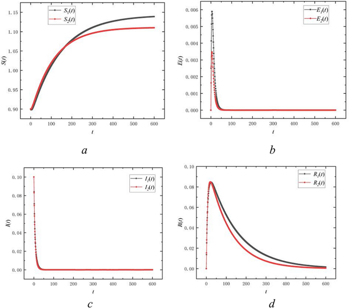
Trends of four types of nodes over time in bilingual environment at \(R_{0} < 1\).
Additionally, the curve of \(I\left( t \right)\) monotonically decreasing nature indicates that the system does not deviate from the disease-free equilibrium but continues to converge towards it over time. This trend aligns with theoretical analyses showing that any small deviations from the disease-free equilibrium will dissipate over time, and in cases where \(R_{0} < 1\), the system will eventually return to a disease-free state.
In the studied model of SEIR public opinion propagation in a bilingual environment, by setting a specific set of parameters:\(\beta_{11} = 0.0028\), \(\beta_{12} = 0.0022\), \(\beta_{21} = 0.0025\),\(\beta_{22} = 0.002\),\(\alpha_{1} = 0.12\),\(\alpha_{2} = 0.11\),\(\gamma_{1} = 0.4\),\(\gamma_{2} = 0.45\),\(d_{1} = 0.001\),\(d_{2} = 0.009\),\(b_{1} = 0.003\), \(b_{2} = 0.003\), \(\mu_{12} = 0.011\), \(\eta_{21} = 0.0015\), \(\mu_{21} = 0.009\), \(\eta_{12} = 0.0017\), and by setting six initial conditions. We simulate the dynamics of public opinion propagation and analyze the global stability of the disease-free equilibrium points when \(R_{0} < 1\). Figure 3 depicts the dynamics of public opinion propagation under various scenarios, each characterized by distinct initial conditions. Specifically, it tracks the trajectory of the proportion of susceptible individuals \(S\left( t \right)\) against the combined proportion of infectious individuals \(I_{1} \left( t \right) + I_{2} \left( t \right)\) over time.
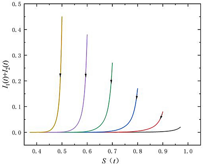
Global asymptotic stability of the disease-free equilibrium points at \(R_{0} < 1\).
Figure 3 displays a series of curves originating from various starting points that converge over time towards common regions. This common region corresponds to the disease-free equilibrium points, where the proportion of infectious individuals approaches zero and the proportion of susceptible individuals remains constant. This trend indicates the global stability of the disease-free equilibrium points when the basic reproduction number (average new infections generated by an infectious individual during their infectious period) is less than 1. A basic reproduction number below 1 signifies that each infectious individual transmits the disease to fewer than one person on average, resulting in the epidemic’s decline.
In the SEIR public opinion propagation model in bilingual environment, this global stability implies that irrespective of initial conditions, the system converges to a disease-free equilibrium where no new public opinions propagated. This phenomenon is illustrated by graphical trajectories showing a decreasing proportion of infectious individuals converging to zero and a stable proportion of susceptible individuals over time.
Therefore, numerical simulations confirm that the system’s disease-free equilibrium is globally asymptotic stable when the basic reproduction number is below 1 in the SEIR public opinion propagation model in bilingual environment.
Stability of the endemic disease equilibrium points
In the studied model of SEIR public opinion propagation in bilingual environment, by setting a specific set of parameters:\(\beta_{11} = 0.14\), \(\beta_{12} = 0.07\), \(\beta_{21} = 0.12\),\(\beta_{22} = 0.06\),\(\alpha_{1} = 0.1\),\(\alpha_{2} = 0.1\),\(\gamma_{1} = 0.005\),\(\gamma_{2} = 0.005\),\(d_{1} = 0.007\),\(d_{2} = 0.007\),\(b_{1} = 0.008\),\(b_{2} = 0.008\),\(\mu_{12} = 0.01\),\(\eta_{21} = 0.01\),\(\mu_{21} = 0.01\),\(\eta_{12} = 0.01\),\(S_{1} = 0.97\), \(E_{1} = 0.01\), \(I_{1} = 0.01\), \(R_{1} = 0.01\), \(S_{2} = 0.97\), \(E_{2} = 0.01\), \(I_{2} = 0.01\), \(R_{2} = 0.01\). We observed key features of public opinion dynamics. The basic reproduction number \(R_{0}\), a critical metric for public opinion propagation, exceeds 1 in this model, indicating that each infectious individual propagated the public opinion to more than one person. Figure 4 show that the proportion of susceptible individuals tends to decrease over time, while the proportion of infectious individuals decreases and then stabilize after an initial rise, and the proportion of recovered individuals increases and stabilize. This dynamic suggests that the public opinion persists in the population and reaches a state of endemic equilibrium under the parameter settings considered. The global asymptotic stability of this equilibrium is evidenced by stable, non-zero proportions of infectious individuals, suggesting that the public opinion will continue to propagated long-term without self-extinguishing. Our analysis indicates that the endemic disease equilibrium points achieves global asymptotic stability when \(R_{0} > 1\), ensuring that the public opinion propagation level remains stable without further interventions.
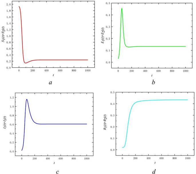
Trends of four types of nodes over time in bilingual environment at \(R_{0} > 1\).
Optimal management
The SEIR public opinion propagation model with management measures in a bilingual environment is Eq. (9); the parameter values can be found in Table 1 below, and take \(B_{1} = 1\), \(B_{2} = 1\), \(B_{3} = 2\), \(B_{4} = 2\), \(B_{5} = 3\), \(B_{6} = 3\). Figures 5, 6, 7 gives the density change of each populations over time in the three scenario. It should be noted that under optimal management , the density of susceptible \(S_{i} \left( t \right)\) and recovered individuals \(R_{i} \left( t \right)\) increases, whereas the density of infectious \(I_{i} \left( t \right)\) and latent individuals \(E_{i} \left( t \right)\) rapidly decreases and stabilizes more quickly. Furthermore, the graph illustrates that management intensity gradually escalates from zero at the onset, reaches a peak, and subsequently declines to zero or to a minimal level.From the figure, it can be seen that the two optimal management strategies are effective in managing public opinion propagation in bilingual environments.
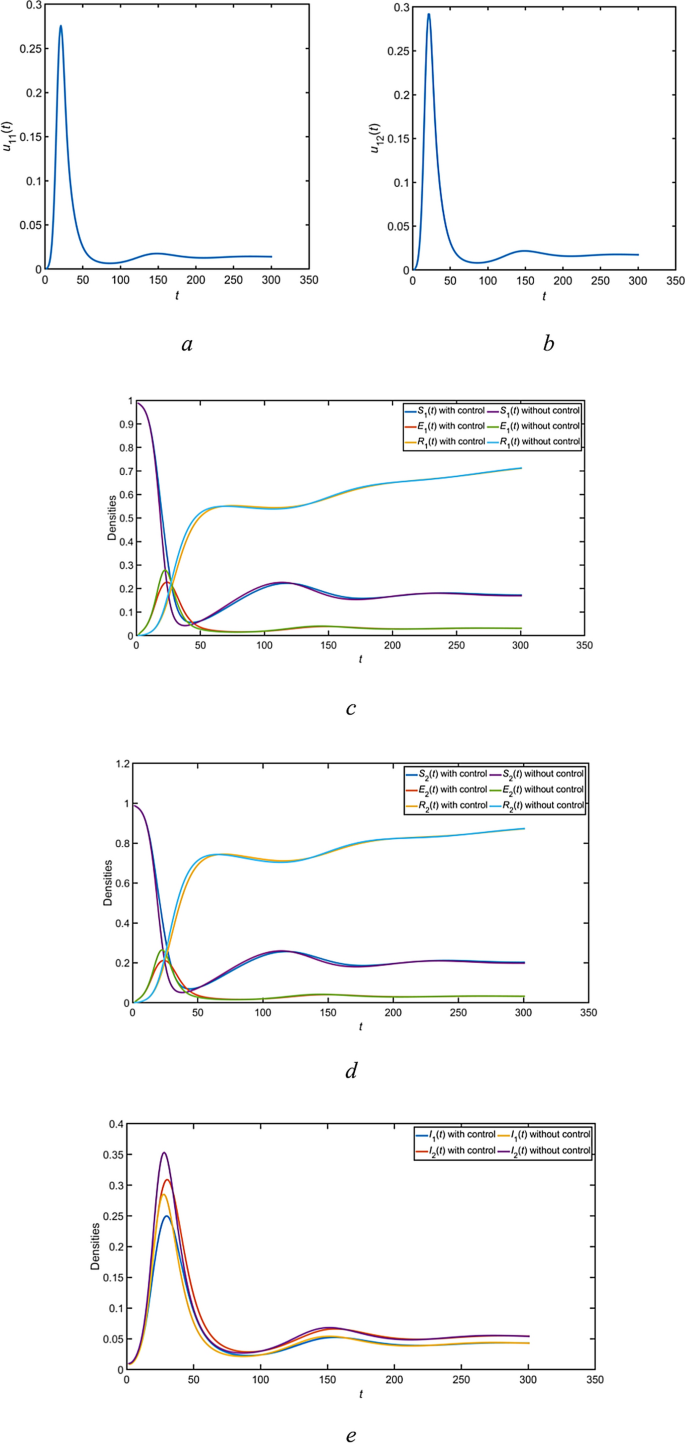
The dynamic of \(S_{i} \left( t \right)\), \(R_{i} \left( t \right)\), \(I_{i} \left( t \right)\), \(E_{i} \left( t \right)\) and management trajectories for the first scenario(\(u_{11} > 0\), \(u_{12} > 0\), \(u_{21} = 0\), \(u_{22} = 0\)).
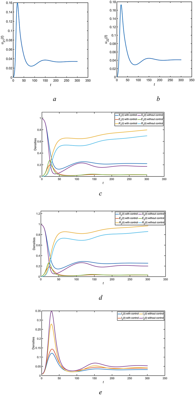
The dynamic of \(S_{i} \left( t \right)\), \(R_{i} \left( t \right)\), \(I_{i} \left( t \right)\), \(E_{i} \left( t \right)\) and management trajectories for the second scenario(\(u_{11} = 0\), \(u_{12} = 0\), \(u_{21} > 0\), \(u_{22} > 0\)).
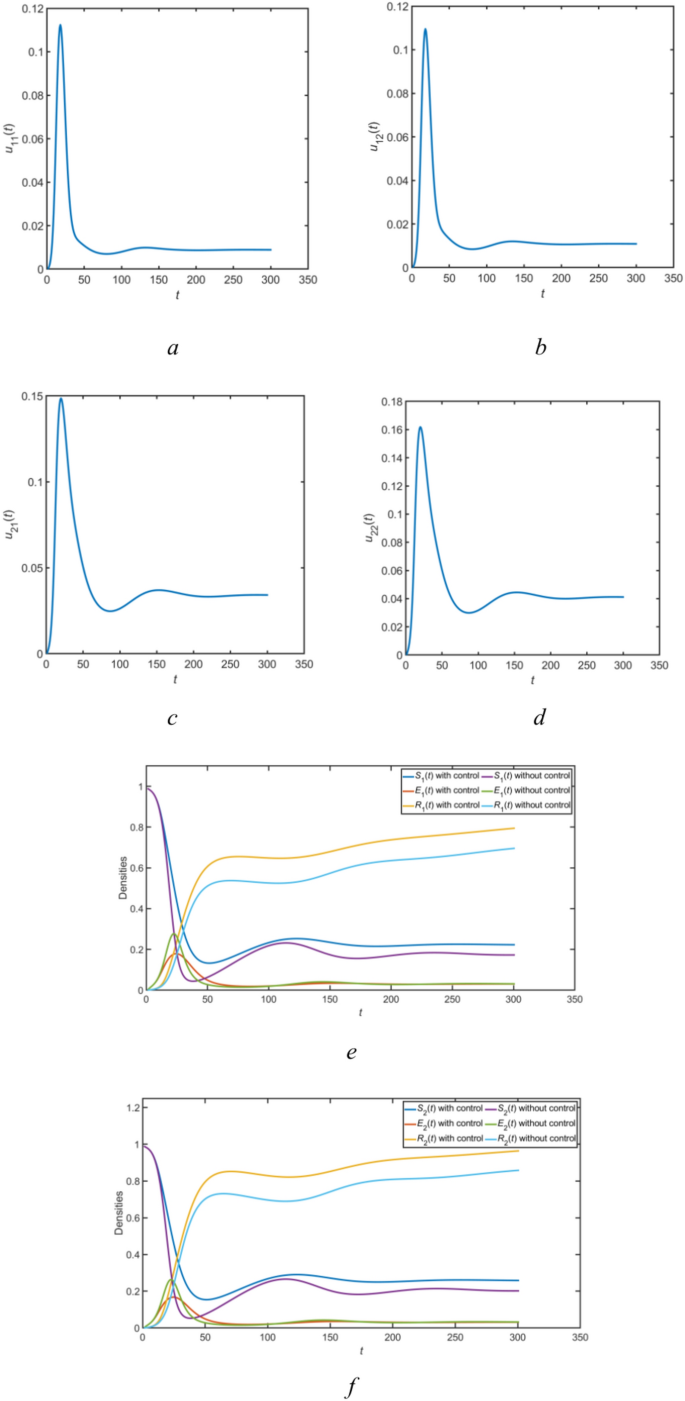
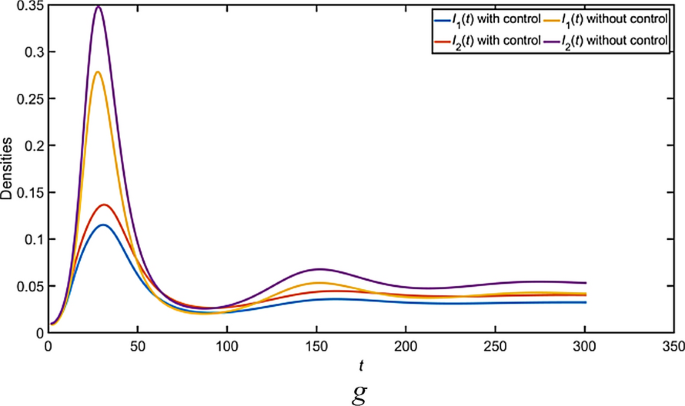
The dynamic of \(S_{i} \left( t \right)\), \(R_{i} \left( t \right)\), \(I_{i} \left( t \right)\), \(E_{i} \left( t \right)\) and management trajectories for the third scenario(\(u_{11} > 0\), \(u_{12} > 0\), \(u_{21} > 0\), \(u_{22} > 0\)).
Model parameter analysis
The effect of propagation rate on the propagation of public opinion
To examine the effect of propagation rate \(\beta_{11}\) on public opinion, we use the data from Table 2 for numerical simulations. We hold all other parameter values constant and vary the propagation rate \(\beta_{11}\) at 0.1, 0.3, 0.5, 0.7, and 0.9. Figure 8a shows how the total infectious individuals \(I_{1} + I_{2}\) varies between bilingual groups at different \(\beta_{11}\) values. The figure illustrates that as \(\beta_{11}\) increases, the peak of public opinion contagion rises and occurs more rapidly. Consequently, a higher contagion rate results in a quicker and broader dissemination of public opinion within the first linguistic group.
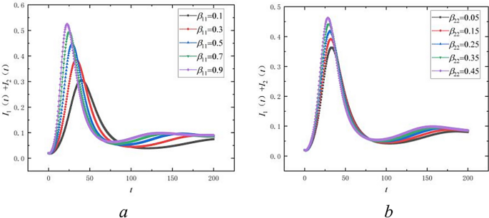
Effect of propagation rate on the propagation of public opinion.
To assess the effect of the propagation rate \(\beta_{22}\) on public opinion, we utilized data from Table 2 for numerical simulations, keeping all other parameter values constant and setting \(\beta_{22}\) at 0.05, 0.15, 0.25, 0.35, and 0.45. Figure 8b illustrates the effects of varying \(\beta_{22}\) values on public opinion propagation within the second linguistic group. As with \(\beta_{22}\), increasing its value not only raises the peak but also accelerates the rate of opinion propagation, suggesting that both the speed and extent of propagation in the second linguistic group intensify with higher propagation rates.
The effect of cross-transmission mechanisms on the propagation of public opinion
To analyze the effect of the cross-transmission rate \(\beta_{12}\) on public opinion, we conducted numerical simulations using data from Table 2. All other parameters remained constant while \(\beta_{12}\) varied at 0.1, 0.3, 0.5, 0.7, and 0.9. Figure 9a illustrates how the total infectious individuals \(I_{1} + I_{2}\) respond in bilingual groups at various \(\beta_{12}\) values. The data indicate that higher \(\beta_{12}\) values accelerate the rate of public opinion propagation, particularly in the first language group, resulting in more rapid propagation and higher peak values. Increased propagation speeds result in infectious individuals propagate public opinions more rapidly, thereby shortening the duration of propagation. This acceleration is due to the enhanced \(\beta_{12}\) value facilitating faster transmission of opinions between the second and first language groups, thereby expediting public opinion propagation in the first language group.
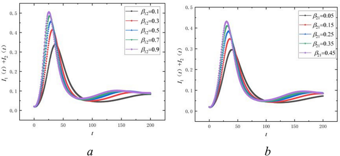
Effect of cross-transmission mechanisms on the propagation of public opinion.
To investigate the effect of cross-transmission rate \(\beta_{21}\) on public opinion, we used data from Table 2 for numerical simulations with all other parameters held constant. \(\beta_{21}\) was set at values of 0.05, 0.15, 0.25, 0.35, and 0.45. Figure 9b illustrates the effect of various \(\beta_{21}\) values on public opinion propagation in bilingual groups. This Figure illustrates that increasing \(\beta_{21}\) values accelerate the propagation of public opinion in the second language group. Additionally, a faster propagation speed results in higher peak levels of opinion spread. The acceleration of opinion propagation in this group is directly attributed to the increased \(\beta_{21}\) values, which enhance the speed of spread.
The effect of social enhancement effects on the propagation of public opinion
When examining the impact of the social enhancement effect \(\eta_{12}\) on public opinion propagation, we conduct numerical simulations using the data from Table 2, keeping other parameter values unchanged. The values of \(\eta_{12}\) are selected as -0.04, -0.025, -0.015, 0, 0.15, 0.025, and 0.04. Equation (2) shows that \(\eta_{12}\) can be negative, zero, or positive, representing the following: \(\eta_{ij} > 0\) indicates that the \(j\)-th language population facilitates opinion propagation in the \(i\)-th language population;\(\eta_{ij} < 0\) indicates inhibition of public opinion propagation from the \(j\)-th language to the \(i\)-th language population; \(\eta_{ij} = 0\) indicates no effect on public opinion propagation between the different language groups. From Fig. 10a, we observe changes in the infectious individuals \(I_{1}\) within the first language group across different \(\eta_{12}\) values. Specifically, as \(\eta_{12}\) increases (from negative to positive), there is an advancement and increase in the peak number of infectious individuals \(I_{1}\) within the first language group. This indicates that a positive \(\eta_{12}\) value suggests a facilitating effect of the second language group on public opinion contagion agents within the first language group. Conversely, a decrease in \(\eta_{12}\)(from positive to negative values) delays and reduces the peak of \(I_{1}\), demonstrating an inhibitory effect. In Fig. 10b, we observe the variation of the infectious individuals \(I_{2}\) within the second language group across different values of \(\eta_{12}\). When \(\eta_{12} = 0\), it indicates negligible opinion contagion interaction between groups. Similarly to \(I_{1}\), the dynamics of infectious individuals in the second language group are affected by the change in \(\eta_{12}\), albeit opposite to the effect on \(I_{1}\); that is, with \(\eta_{12}\) (from negative to positive values), there is a delay and decrease in the peak number of infectious individuals \(I_{2}\) in the second language group.
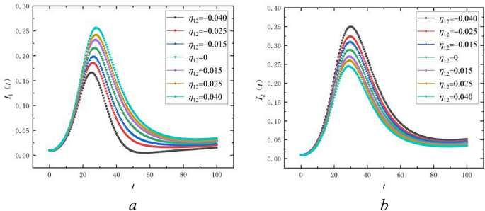
Social Enhancement Effect \(\eta_{12}\) on the propagation of public opinion.
When analyzing the impact of the social enhancement effect \(\eta_{21}\) on public opinion propagation, we conducted numerical simulations using the data from Table 2. Other parameters in Table 2 remained constant, while \(\eta_{21}\) was varied at values of -0.04, -0.025, -0.015, 0, 0.15, 0.025, and 0.04. From Fig. 11a, we observe the variation of \(I_{1}\) in the first language group under different values of \(\eta_{21}\). Specifically, as \(\eta_{21}\) increases from negative to positive values, there is an advancement and increase in the peak number of infectious individuals \(I_{2}\) in the second language group. This indicates that when \(\eta_{21} > 0\) the first language group facilitates opinion contagion in the second language group. Conversely, as \(\eta_{21}\) decreases from positive to negative values, the peak of \(I_{2}\) is delayed and decreases, indicating an inhibitory effect. Figure 11b illustrates the variation of infectious individuals \(I_{1}\) in the first language group across different \(\eta_{21}\) values. Similarly to \(I_{2}\), we observe a trend where changes in \(\eta_{21}\) affect the dynamics of infectious individuals in the first language group. However, this effect is opposite to that observed for \(I_{2}\); specifically, there is a delay and decrease in the peak number of infectious individuals \(I_{1}\) within the first language group as \(\eta_{21}\) transitions from negative to positive values.
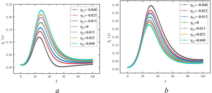
Social Enhancement Effect \(\eta_{21}\) on the propagation of public opinion.
The impact of social enhancement effects on Public Opinion Propagation in multilingual environment involves multiple interacting factors, such as foundational influence capacity, cultural proximity, contagion proportion, and threshold parameters. Foundational influence capacity reflects the basic level of interaction among diverse linguistic groups without further social or cultural influences. Higher values correlate with linguistic similarities, frequent communication, and positive historical interactions, facilitating faster information dissemination. Cultural proximity evaluates whether cultural similarities facilitate or impede information flow. Closer cultural ties lead to more efficient information dissemination, enhancing the spread of public opinion.
The contagion proportion indicates the percentage of group members actively involved in public opinion propagation. A higher contagion proportion signifies increased activity in disseminating information, which can amplify the impact of public opinion. The threshold parameter determines whether the social enhancement effect fosters, inhibits, or has no impact on Public Opinion Propagation, highlighting crucial conditions for inter-group interaction. When the contagion proportion exceeds the threshold, it promotes faster dissemination of public opinion; conversely, falling below the threshold can impede dissemination due to disparities in information acceptance or cultural isolation.
Therefore, the direction and magnitude of social enhancement effects directly influence the speed and scope of Public Opinion Propagation among diverse linguistic groups. These factors collectively reveal the complex mechanisms of Public Opinion Propagation in multilingual societies and provide new insights and strategies for opinion management in multicultural settings.
The effect of forgetting mechanism on the propagation of public opinion
When examining the impact of the forgetting mechanism \(\mu_{12}\) on public opinion propagation, we utilized the data from Table 2 for numerical simulation, maintaining the constant values of other parameters. The values of \(\mu_{12}\) were chosen as follows: 0.05, 0.15, 0.25, 0.35, and 0.45. From Fig., we observe the variation of the total infectious individuals \(I_{1} + I_{2}\) across different values of \(\mu_{12}\) in the bilingual groups. As depicted in Fig. 12a, \(I_{1} + I_{2}\) represents the temporal evolution of the total number of infectious individuals across bilingual groups. With an increase in \(\mu_{12}\), we note a decrease in the peak value of \(I_{1} + I_{2}\) along with its rightward shift, signifying the attenuation of the speed and breadth of public opinion propagation due to the forgetting effect. The elevation of \(\mu_{12}\) decelerates the pace and extent of public opinion propagation within the first language group.
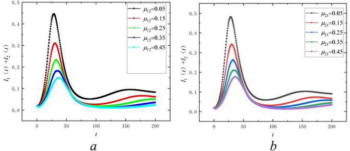
The effect of forgetting mechanism on the propagation of public opinion.
When examining the impact of the forgetting mechanism \(\mu_{21}\) on public opinion propagation, we utilize the data from Table 2 for numerical simulation, maintaining constant values for other parameters. The values of \(\mu_{21}\) are as follows: 0.05, 0.15, 0.25, 0.35, and 0.45. Figure 12b illustrates the variations in the total infectious individuals \(I_{1} + I_{2}\) across the bilingual groups at different \(\mu_{21}\) values. As depicted in Fig. 12b, an increase in \(\mu_{21}\) results in a decrease in the peak value of \(I_{1} + I_{2}\), accompanied by a rightward shift, indicating once more that the speed of opinion propagation and its influence are curbed by the forgetting effect. The elevation of \(\mu_{21}\) decelerates the propagation speed and breadth of public opinion within the second language group.
These simulation results clearly show the impact of factors like base forgetting rate, adjustments in cross-linguistic social enhancement effects, cultural proximity, and information quality on the forgetting mechanism in a multilingual setting. The base forgetting rate indicates the natural rate at which different linguistic groups forget information, unaffected by external factors. This ratio is influenced by cognitive ability, information complexity, and frequency of exposure. Meanwhile, the cross linguistic social enhancement effect indicates that communication frequency, understanding level, and information resonance between language groups can accelerate or slow down the rate of forgetting. Cultural similarity improves the efficiency of information dissemination, reduces forgetting rates, and enables culturally similar groups to more effectively retain information. The quality of information, especially its reliability and relevance, can effectively affect the retention of information over time, slowing down the rate of information forgetting.
Over time, with the continuous influx of new information and limited attention, old information is gradually forgotten. However, influenced by the factors mentioned earlier, this forgetting process varies greatly among different language groups. It not only affects the absorption capacity of information, but also affects the formation and dissemination process of public opinion. These findings highlight the necessity of considering these factors in global cross-cultural interaction.
The impact of asymmetric initial conditions on multilingual Public Opinion Propagation
In this simulation, we constructed a bilingual Public Opinion Propagation model with initial conditions set as asymmetric dissemination scenarios. Specifically, the susceptibility of the second language group is 100% (\(S_{2} = 1\)), with 0 initial infected individuals (\(I_{2} = 0\)), while the first language group has a certain proportion of initial infected individuals (\(I_{1} = 0.05\)). The values of other parameters are shown in Table 3. This setting aims to simulate certain language groups being unaffected by public opinion in the early stages due to cultural isolation, information barriers, or limitations in communication channels, while another language group has already begun to spread public opinion. The design of such asymmetric initial conditions helps us understand how cross linguistic communication and information lag affect the dynamic evolution of two language groups in the process of Public Opinion Propagation.
From Fig. 13a, it can be seen that there are significant differences in the dissemination patterns of public opinion between the two language groups: the first language group (\(S_{1}\), \(E_{1}\), \(R_{1}\)): Initially, due to the presence of infected individuals (\(I_{1} = 0.05\)), public opinion spreads rapidly in the first language group. As the number of infected individuals increases, the number of susceptible individuals (\(S_{1}\)) rapidly decreases, and the spread of public opinion enters the incubation period (\(E_{1}\)), gradually reaching its peak. As time goes by, the number of infected individuals decreases and the number of recovered individuals (\(R_{1}\)) gradually increases, indicating a gradual decline in public opinion. The restorer curve (\(R_{1}\)) shows that over time, public opinion in this language group has been effectively controlled and eventually stabilized. Second language groups (\(S_{2}\), \(E_{2}\), \(R_{2}\)): In contrast, due to the initial lack of infected individuals, the dissemination of public opinion in the second language group is significantly lagging behind. Public opinion spreads across languages from the first language group to the second language group (through parameters such as \(\beta_{12}\) and \(\beta_{21}\)). After a certain period of time, the susceptible individuals (\(S_{2}\)) in the second language group are gradually affected, and the transmission curve begins to emerge, with \(E_{2}\) and \(R_{2}\) starting to change. Eventually, the spread of public opinion among the second language group gradually reached its peak and then entered a period of recovery.
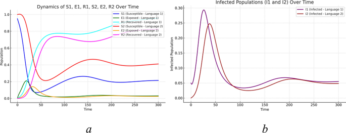
The impact of asymmetric initial conditions on multilingual Public Opinion Propagation.
This asymmetric dissemination pattern indicates that there is a significant cross linguistic communication lag phenomenon in the dissemination of public opinion. Due to the initial lack of infected individuals, the second language group was largely unaffected in the early stages of Public Opinion Propagation. However, with the passage of time and the strengthening of cross linguistic transmission effects, this group eventually entered the cycle of Public Opinion Propagation.
Figure 13b shows the changes in the number of infected individuals (\(I_{1}\), \(I_{2}\)) in two language groups over time, further revealing the asymmetry of Public Opinion Propagation:\(I_{1}\) curve (infected individuals in the first language group): At the beginning, the number of infected individuals rapidly increases and reaches a peak in a short period of time, then gradually decreases and tends to stabilize. This trend reflects the rapid spread of public opinion within the first language community and the subsequent decrease in the number of infected individuals due to recovery or management measures. \(I_{2}\) curve (infected individuals in the second language group): In contrast, the infected individuals curve in the second language group lags significantly behind. The number of infected individuals only began to significantly increase after a certain period of time, indicating that public opinion gradually expanded to the second language group through cross linguistic transmission. In the end, the trend of \(I_{2}\) changes is consistent with \(I_{1}\), but the entire propagation process is significantly lagging behind.
This phenomenon reveals the delayed effect of information transmission across languages. The increase in the number of infected individuals in the second language group is limited by interaction with the first language group (through cross linguistic transmission parameters) due to being in a completely susceptible state in the initial stage. As the public opinion of the first language group gradually enters a stable period, the number of infected individuals in the second language group begins to increase significantly.
The simulation results reveal the complexity of cross linguistic communication from the perspective of dynamic propagation. In reality, certain language groups may exhibit significant lag in the early stages of Public Opinion Propagation due to cultural isolation or differences in information dissemination channels. For example, certain language groups may not have received sufficient public opinion information in the first instance during a specific event, resulting in them starting to be influenced by public opinion after a longer period of time. On the other hand, the cross linguistic dissemination rate is reflected in the model through the \(\beta_{12}\) and \(\beta_{21}\) parameters, which simulate the social interaction intensity and information transmission efficiency between different language groups.
This model is of great significance to policy makers, social media platforms and public crisis managers. By understanding the lag effect in multilingual public opinion communication, relevant departments can formulate targeted emergency measures in advance, and carry out phased public opinion management and guidance based on the communication characteristics of different language groups.
The impact of network structure on the process of public opinion
To verify the impact of complex network topology on the process of public opinion propagation, three typical network structures were selected for comparison. Using the NetLogo software, simulation experiments were conducted on the SEIR-based public opinion propagation model in a bilingual environment across three networks: a regular network (4000 nodes, 16,000 edges), a WS small-world network (4000 nodes, 16,000 edges), and a BA scale-free network (4000 nodes, 8000 edges). As shown in Fig. 14, the visualization of these three classical complex networks is presented. The parameter settings are shown in Table 4.
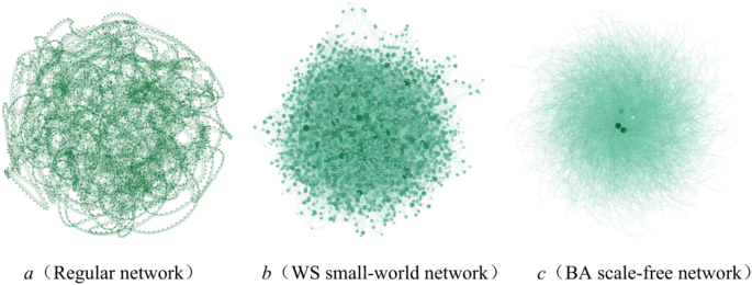
Visualization of three types complex networks.
Figure 15 simulates the temporal evolution of the densities of two different language propagators,\(I_{1}\) and \(I_{2}\), within three different network topologies. Figure 15a illustrates the propagation process of language 1 propagators across the three networks. The black curve represents the scale-free network, the red curve represents the small-world network, and the blue curve represents the regular network. The overall trend shows that all three curves initially rise to a peak, then decline, and eventually stabilize. As depicted, the black curve reaches the highest peak, followed by the blue curve, and the red curve has the lowest peak, but the red curve stabilizes the earliest. Figure 15b depicts the propagation process of language 2 propagators across the three networks. Similarly, the black curve represents the scale-free network, the red curve represents the small-world network, and the blue curve represents the regular network. In Fig. 14b, the differences in peak values among the three curves are even more pronounced, with the black curve having the highest peak, the blue curve the second highest, and the red curve the lowest. Again, the red curve stabilizes the earliest. The underlying reason is that the BA scale-free network is characterized by a power-law distribution of node connections, where the majority of nodes have few connections, while a few hub nodes have a large number of connections. These hub nodes play a critical role in the spread of public opinion, leading to the highest rise in propagator density. The small-world network, which lies between a completely regular network and a completely random network, introduces a small probability of long-distance connections by rewiring the original nearest-neighbor nodes. This network structure is characterized by most nodes being locally connected, with occasional long-distance connections, which facilitates the rapid spread of public opinion information.
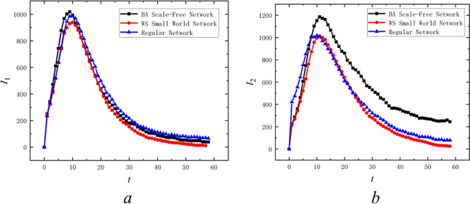
The Impact of network structure on the process of public opinion.
Validation of the model on the Twitter dataset
In this section, we utilize a real dataset from Twitter51 to evaluate the effectiveness of the proposed model. As of September 2021, this dataset contains over 2.2 billion tweets collected since January 22, 2020, covering discussions about COVID-19 and published in multiple languages. Among these multilingual tweets, English tweets have the highest proportion, followed by tweets in Spanish and Catalan. Consequently, we selected data from tweets related to COVID-19, published in English, Spanish, and Catalan during the first 100 days from January 22, 2020, as the dataset to validate the SEIR opinion propagation model proposed in this paper under a bilingual environment. Given the large volume of data, we define a user as an opinion spreader only if they post tweets related to COVID-19 in English, Spanish, or Catalan, without considering the number of likes received. As shown in Table 5, each column of the dataset contains specific information related to individual tweets and retweets. This information includes user ID, timestamp corresponding to the date and time of each tweet or retweet, the language used for the tweet, the status of the tweet, and other relevant details.
We employ the SEIR opinion propagation model under a bilingual environment, fitting \(I_{1}\) to represent the temporal dynamics of English opinion spreaders on Twitter and \(I_{2}\) to represent the temporal dynamics of Spanish and Catalan opinion spreaders. According to Twitter user data,52 the daily active user count on Twitter in 2020 was 192 million, an increase from 152 million in 2019. Therefore, we assume that each user posts only one tweet per day and use this assumption to calculate the proportion of English tweets relative to the total daily active users, thereby estimating the proportion of English opinion spreaders. A similar method is applied to estimate the proportion of Spanish and Catalan opinion spreaders. The parameter settings for the fitting process are detailed in Table 6, and the fitting results are illustrated in Fig. 16.
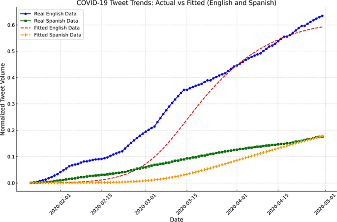
Fitting effect of Twitter real dataset.
Figure 16 illustrates the model’s ability to capture the dynamics of public opinion propagation in a multilingual context, focusing on English and Spanish tweet activity related to COVID-19. The blue and green curves represent the actual tweet volumes in English and Spanish, respectively, while the red and orange dashed curves reflect the SEIR model’s fitted results. The model incorporates three critical mechanisms: social enhancement, forgetting, and cross-transmission.
As shown in the figure, the model effectively fits the Spanish tweet data throughout both the early and later stages of the propagation process, demonstrating the influence of social enhancement—where active opinion spreaders amplify their impact within smaller, more homogenous language groups. In contrast, the forgetting mechanism, which accounts for the decay of engagement over time, is more evident in the English data, where the higher volume of tweets leads to more complex and unpredictable behavior, particularly in the later stages.
In conclusion, the SEIR opinion propagation model, applied within a bilingual environment, has demonstrated its effectiveness in capturing the dynamics of public opinion across multiple languages. The model shows particularly strong performance in fitting the propagation trends of Spanish and Catalan tweets, where opinion dynamics are more consistent and predictable. This superior fitting underscores the model’s ability to adapt to smaller, more homogeneous linguistic groups, which exhibit less variability in opinion spread over time.
Compared to single-language models, the bilingual SEIR model offers a more comprehensive reflection of opinion propagation in multilingual and multicultural contexts. It captures the nuances of cross-transmission between languages, social enhancement within linguistic communities, and the decay of engagement through the forgetting mechanism. These features not only improve the model’s precision and reliability but also highlight its capability to account for the complexities inherent in multilingual environments.
This multilingual modeling approach broadens the model’s applicability, enhancing its practicality for global opinion analysis. By incorporating diverse linguistic and cultural dynamics, the model becomes a valuable tool for more accurate and inclusive public opinion management in increasingly interconnected and multicultural societies.


